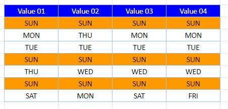
Highlight Duplicate Rows – Excel & Google Sheets

This tutorial will demonstrate how to highlight duplicate rows using Conditional Formatting in Excel and Google Sheets.

Highlight Duplicate Rows – COUNTIFS Function

To highlight duplicate rows with Conditional Formatting, use the COUNTIFS Function within a Conditional Formatting rule.

When programmed properly, the COUNTIFS Function will count all rows that match the current row.

Note: If you simply want to highlight duplicate values (instead of rows), you can use Excel’s built-in Highlight Cells Rules > Duplicate Cell Values.

1. Select the range you want to apply formatting to.
2. In the Ribbon, select Home > Conditional Formatting > New Rule.

3. Select Use a formula to determine which cells to format, and enter the COUNTIFS formula:

=COUNTIFS($B$4:$B$10,$B4,$C$4:$C$10,$C4,$D$4:$D$10,$D4,$E$4:$E$10,$E4)>1

Note: Your formula will differ based on the number of columns to compare.

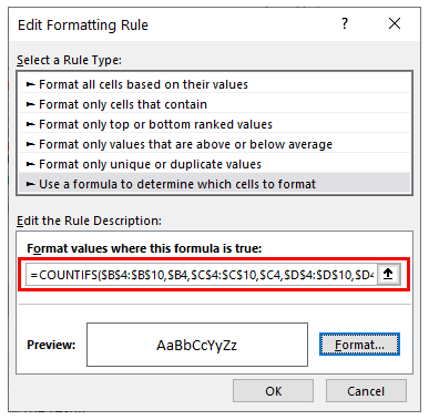
4. Click on the Format button and select your desired formatting.

5. Click OK to view the result.

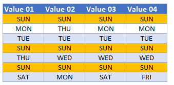
Highlight Duplicate Rows in Google Sheets

The process to highlight duplicate rows in Google Sheets is similar to the process in Excel.

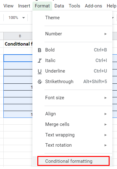
1. Highlight the cells you wish to format, and then click on Format > Conditional Formatting.

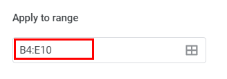
2. The Apply to Range section will already be filled in.

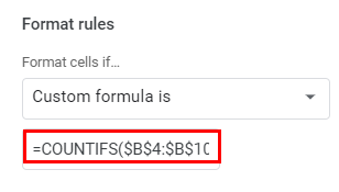
3. From the Format Rules section, select Custom Formula from the drop-down list and type in the formula:

=COUNTIFS($B$4:$B$10,$B4,$C$4:$C$10,$C4,$D$4:$D$10,$D4,$E$4:$E$10,$E4)>1

4. Select the fill style for the cells that meet the criteria.

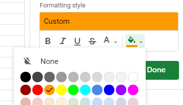
5. Click Done to apply the rule.