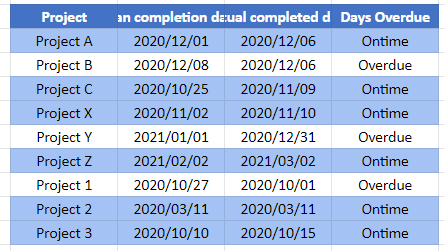
Highlight Rows That Contain – Excel & Google Sheets

This tutorial will demonstrate how to highlight rows where a cell in that row contains a certain value using Conditional Formatting in Excel and Google Sheets.

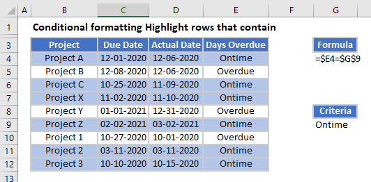
Highlight Cells That Contain…

You can highlight cells that contain a certain value by creating a Conditional Formatting rule and creating a custom formula.

1. Select the range you want to apply formatting to.
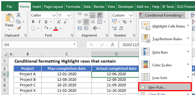
2. In the Ribbon, select Home > Conditional Formatting > New Rule.

3. Select Use a formula to determine which cells to format, and enter the formula:

=$E4=$G$9

You need to use a mixed reference in this formula ($E4) in order to lock the column but make the row relative – this will enable the formatting to format the entire row instead of just a single cell that meets the criteria.

When the rule is evaluated for all the cells in the range, the row will change but the column will remain the same. This causes the rule to ignore the values in any of the other columns and just concentrate on the values in Column E. As long as the rows match, and Column E of that row contains the word Ontime, then the formula result is TRUE and the formatting is applied for the whole row.

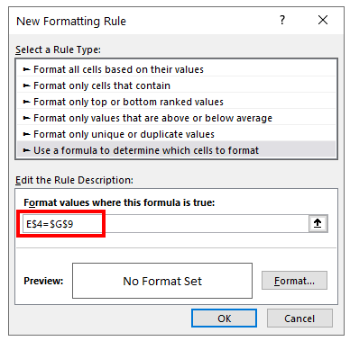
4. Click on the Format button and select your desired formatting.

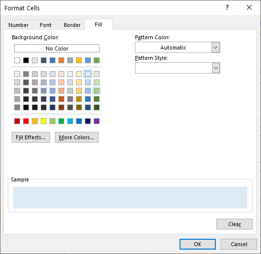
5. Click OK and then OK again to view the result.

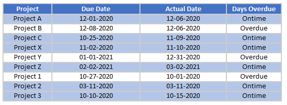
Highlight Cells that Contain… in Google Sheets

The process to highlight rows where one of the cells in the row meets the given criteria in Google Sheets is similar to the process in Excel.

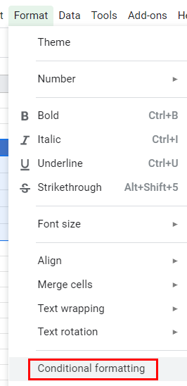
1. Highlight the cells you wish to format, and then click on Format > Conditional Formatting.

2. The Apply to Range section will already be filled in.

1. From the Format Rules section, select Custom Formula from the drop-down list and type in the following formula:

=$E4=$G$9

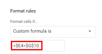
4. Once again, you need to use the dollar signs to lock in the column but not the row thereby creating a mixed reference.
5. Select the fill style for the cells that meet the criteria.

6. Click Done to apply the rule.