Average If Not Blank – Excel & Google Sheets
Download the example workbook
This tutorial will demonstrate how to calculate the average of a set of numbers while ignoring blank values or categories in Excel and Google Sheets.
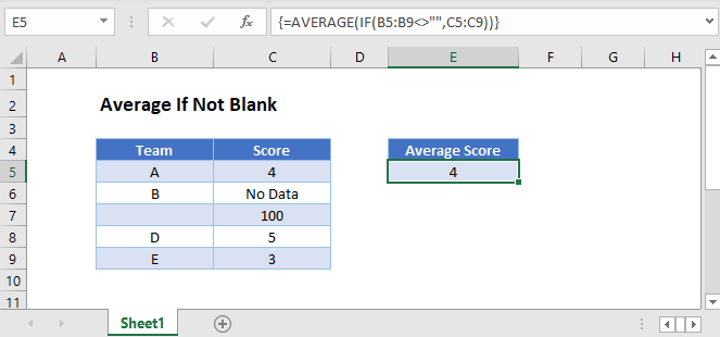
Ignore Blank Values with AVERAGE Function
The AVERAGE Function automatically ignores any cells that are blank or that contain text.
This example uses the AVERAGE Function to calculate the Average Score, which will ignore the text and blank values in column C:
=AVERAGE(C3:C7)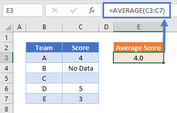
Treat Text Values as Zero with AVERAGEA Function
In order to treat text values as zero in the calculation, use the AVERAGEA Function.
Notice how this example includes the text value “No Data” in the average calculation.
=AVERAGEA(C3:C7)
This example calculates the average of the values 4, 0, 5 and 3
Ignore Blank Category Values Using AVERAGEIFS
This example uses the AVERAGEIFS Function to calculate the Average Score for teams with non-blank names and ignores Scores that are text values.
=AVERAGEIFS(C3:C7,B3:B7,"<>")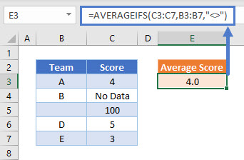
Ignore Blank Category Values – Array
If you don’t have access the AVERAGEIF function, you can use a nested AVERAGE and IF Function.
This example calculates the Average Score for teams with non-blank names and ignores any Scores that is a text value
=AVERAGE(IF(B3:B7<>"",C3:C7))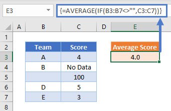
This formula uses the IF Function to evaluate whether the name of each Team is not blank, and only uses Scores from Teams with non-blank names in the AVERAGE Function. The score of 100 is ignored as the Team name is blank. The score of ‘No Data’ is ignored as it is not a numerical value.
In versions of Excel from 2019 and earlier, this formula is required to be entered as an array formula by pressing CTRL + SHIFT + ENTER. This is not required in later versions
This example can equally be calculated using an AVERAGEIFS Function as shown below
Ignore Blank Category Values and Treat Text as 0
In order to treat text value Scores as 0, whilst still ignoring Teams with blank names, we can use a nested AVERAGEA and IF Function:
=AVERAGEA(IF(B3:B7<>"",C3:C7))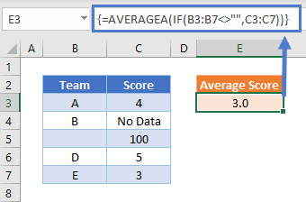
This formula uses the IF Function to evaluate whether the name of each Team is not blank, and only uses Scores from Teams with non-blank names in the AVERAGEA Function. The score of 100 is ignored as the Team name is blank. The score of ‘No Data’ is treated as 0 by the AVERAGEA Function and so an average of 3.0 is calculated.
In versions of Excel from 2019 and earlier, this formula is required to be entered as an array formula by pressing CTRL + SHIFT + ENTER. This is not required in later versions
Average If Not Blank in Google Sheets
Most of these formula examples work in the same way in Google Sheets as in Excel, but with some exceptions:
Whenever an IF Function is nested within another function and it references a cell range, Google Sheets needs to treat the formula as an array formula by using the ARRAYFORMULA Function:
=ArrayFormula(AVERAGE(IF(B3:B7<>"",C3:C7)))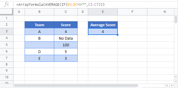
The AVERAGEA Function works differently in Google Sheets and so the example of =AVERAGEA(IF(B3:B7<>””,C3:C7)) cannot be used. This is because when the IF Function finds a blank value in the B3:B7 range, it produces a null value, which Google Sheets counts as 0 instead of ignoring it like in Excel.