Find Last Row – Excel & Google Sheets

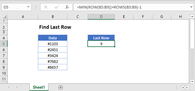
This tutorial will demonstrate how to find the number of the last row in a range in Excel and Google Sheets.

Find the Last Row of a Range

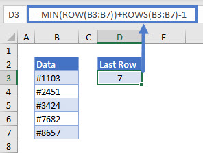
To find the last row of a range, you can use the ROW, ROWS, and MIN Functions:

=MIN(ROW(B3:B7))+ROWS(B3:B7)-1

Let’s see how this formula works.

ROW with MIN Function

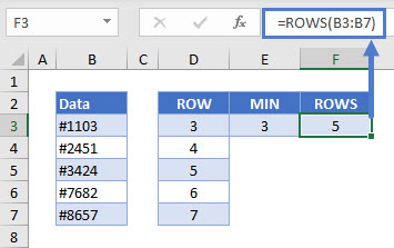
For a range with multiple rows, the ROW Function returns an array that contains all row numbers in that range.

=ROW(B3:B7)

Note: If you are using Excel 2019 or earlier, to create this array formula you must press CTRL + SHIFT + ENTER to close out the formula instead of simply pressing ENTER.

We only need the first row number and can get it with the MIN Function. The MIN Function returns the smallest of a set of numbers.

=MIN(D3:D7)

Here, our range starts on Row 3.

ROWS Function

The ROWS function returns the total number of rows in a range.

=ROWS(B3:B7)

Start with the first row number, add the total number of rows, and subtract 1 to get the row number of the last cell in the range.

=E3+F3-1

This is equivalent to our original formula of:

=MIN(ROW(B3:B7))+ROWS(B3:B7)-1

 

Find Last Row in Google Sheets

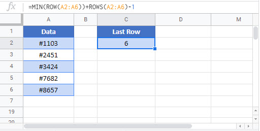
These formulas work exactly the same in Google Sheets as in Excel.