If ISNA & IFNA in VLOOKUPs – Excel & Google Sheets
This tutorial will demonstrate how to handle VLOOKUP #N/A errors in Excel and Google Sheets. If you have access to the XLOOKUP Function, read our article on handling XLOOKUP errors.

IFNA in VLOOKUP
When you lookup a value with the VLOOKUP Function, if the value is not found, VLOOKUP will return the #N/A error.
=VLOOKUP(E3,B3:C6,2,FALSE)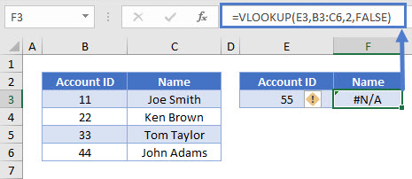
You can add the IFNA Function outside of the VLOOKUP, to do something else if the VLOOKUP results in an IFNA error. In this example, we will output “Not found” if the VLOOKUP results in an #N/A error:
=IFNA(VLOOKUP(E3,B3:C6,2,FALSE),"Not found")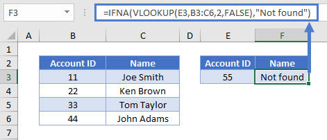
Note: The new XLOOKUP Function has built-in error handling. The IFNA Function is not needed!
Another common use of the IFNA Function is to perform a second VLOOKUP if the first VLOOKUP can not find the value. This may be used if a value could be found on one of two sheets; if the value is not found on the first sheet, lookup the value on the second sheet instead.
=IFNA(VLOOKUP(E3,B3:C6,2,FALSE),VLOOKUP(E3,'Data'!B3:C6,2,FALSE))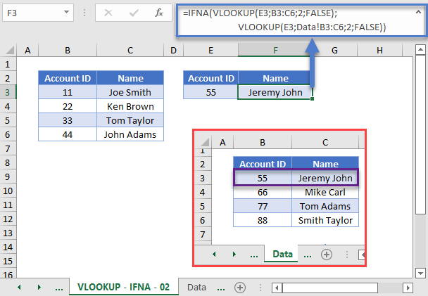
IF ISNA in VLOOKUP
The IFNA Function was introduced in Excel 2013. Prior to that, you had to use the more complicated IF / ISNA combination:
=IF(ISNA(VLOOKUP(E3,B3:C6,2,FALSE)),"Not found",VLOOKUP(E3,B3:C6,2,FALSE))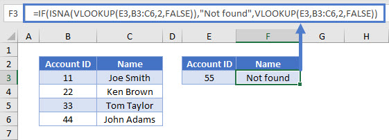
The ISNA function checks whether the result of the VLOOKUP formula is an #N/A error and returns True or False accordingly. If it is true (i.e., your lookup value is missing from the lookup array), the IF function will return with a message you specify, otherwise it will give you the result of the VLOOKUP.
IFERROR – VLOOKUP
As stated above, the IFNA Function tests if the formula outputs only a #N/A error. Instead, the IFERROR Function can be used to check if ANY error is returned:
=IFERROR(VLOOKUP(E3,B3:C6,2,FALSE),"Not found")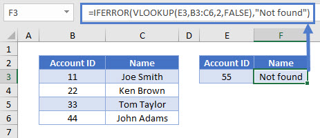
Usually it’s better to use IFNA instead of IFERROR, as IFERROR will handle errors that might need your attention.
If ISNA & IFNA in VLOOKUPs – Google Sheets
These formulas work the same in Google Sheets as in Excel.
