Create Multiplication Table in Excel & Google Sheets
Download the example workbook
In this tutorial, we will learn how to create multiplication in Excel & Google Sheets.
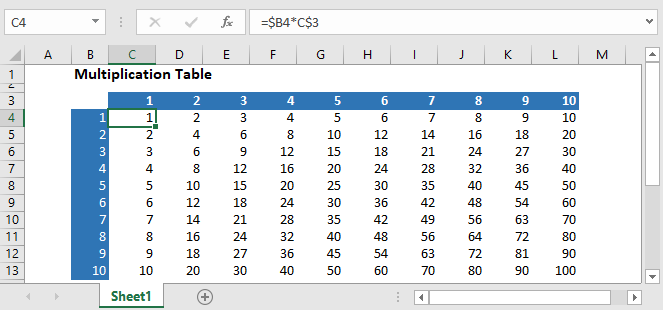
Setting up Data
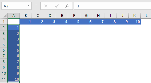
To set up the data, enter numbers 1-10 in cells A2 to A11 and again in cells B1 to K1.
There’s also an interesting way to insert the numbers in the cells, with the TRANSPOSE function:
- Enter the numbers 1-10 in cells A2 to A11.
- Select the range B1:K1 and type the following formula in the formula bar.
- Press Ctrl+Shift+Enter, because it’s an array formula (not necessary in Excel 365 or versions of Excel after 2019).
=TRANSPOSE(A2:A11)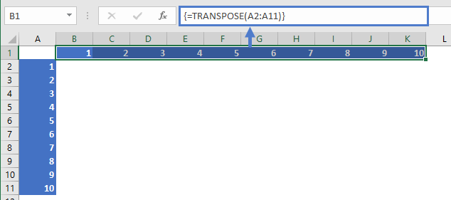
Now we have the set up for our multiplication table. Below we will demonstrate two ways to populate the multiplication table.
Multiplication Table using mixed references
The multiplication table can be created by using mixed cell references, where one either the row or column reference is locked and the other is not.
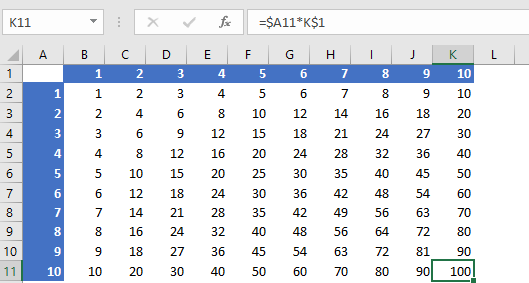
Use this formula in cell B2:
=$A2*B$1
This will lock the header row for number and will multiply the header column row and will return the result.
Then we’ll copy and paste this formula into the entire range:
- Copy cell B2 (Ctrl + C).
- Select the range B2:K11
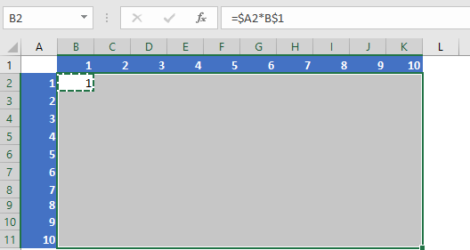
- Press Ctrl+V to paste the formula
Multiplication Table using Array Formula
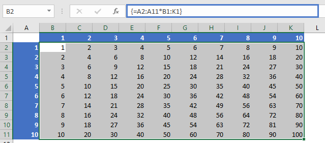
The array formula method is also very simple.
You’ll just have to select the range B1:K1 and insert of the formula in the formula bar and press Ctrl+Shift+Enter (Excel 2019 and Earlier):
=A2:A11*B1:K1
In this way, the whole multiplication table will be created.
Create a Multiplication Table in Google Sheets
The formula to create multiplication table works exactly the same in Google Sheets as in Excel:
