Remove Specific Text From a Cell in Excel & Google Sheets

This tutorial will demonstrate how to remove specific text from a cell in Excel & Google Sheets.

Remove Specific Text

To find and remove specific text in Excel, we can use the SUBSTITUTE function.

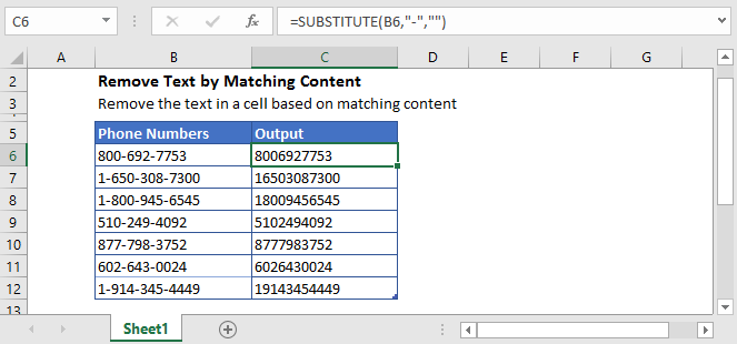
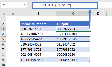
Let’s say we have hyphen signs (“-“) in a text and we want to remove it. We can do this with SUBSTITUTE function by using the following formula:

=SUBSTITUTE(B3,"-","")

In this example, we’ve provided the cell reference (B3), the content we want to remove from the text (“-”), and for replacement text, the empty string (“”).

The SUBSTITUTE function replaces all the hyphens “-” with nothing.

We can remove any other character or text from the main text string by replacing the hyphen sing (“-“) in the formula with that character or text.

Remove more than one Character

We can also remove more than one character from the text by nesting SUBSTITUTE functions.

Let’s say we have parenthesis and hyphens in text and we want to remove them both. We’ll nest SUBSTITUTE functions three times, to get the desired result, like this:

=SUBSTITUTE(SUBSTITUTE(SUBSTITUTE(B3,"(",""),")",""),"-","")

First, the Excel will remove the “(” character from the text, then moves to the outer nested SUBSTITUTE function and removes the “)”, and then proceeds to the further outer SUBSTITUTE function and removes the hyphen sign (“-“).

Remove Text In Google Sheets

The formula to remove the text by matching content works exactly the same in Google Sheets as in Excel: