sum if by day of week – Excel & Google Sheets
Download the example workbook
This tutorial will demonstrate how to use the SUMIFS Function to sum data corresponding to specific days of the week in Excel and Google Sheets.

Sum If by Day of Week – Text Values
First, we will demonstrate how to sum data corresponding to specific Day of Week names.
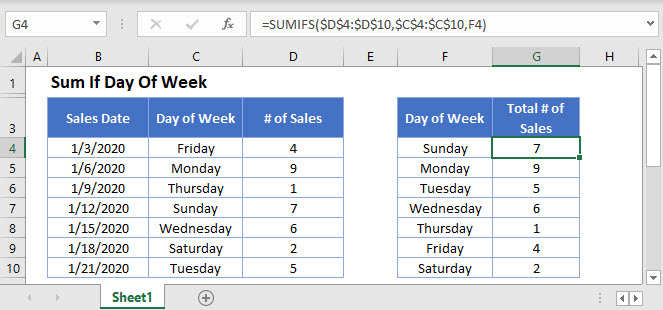
We can use the SUMIFS Function, along with a helper column containing the TEXT Function to sum all Sales that take place on a specific Day of Week:
=SUMIFS(D3:D9,C3:C9,F3)
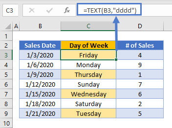
In the above example, we use the TEXT Function to extract the name of the Day of Week from the Sales Date:
=TEXT(B3,"dddd")
The SUMIFS Function then uses this helper column to produce the summary table:
=SUMIFS(D3:D9,C3:C9,F3)
Sum If by Day of Week – Using WEEKDAY
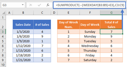
Alternatively, weekday numbers can be used. To do this, the helper column in the source data needs to use the WEEKDAY Function:
=WEEKDAY(B3)
Using the WEEKDAY numerical value instead of the weekday name may provide you with more flexible options for later data visualization tasks and summary functions.
Sum If by Day of Week – Without Helper Column
The above example summed data by weekday using a helper column. To avoid the need for a helper column, we can use the SUMPRODUCT Function:
=SUMPRODUCT(--(WEEKDAY(B3:B9)=E3),C3:C9)
Here, the SUMPRODUCT Function performs a complicated “sum if” calculation. Let’s walk through the above example.
This is our final formula:
=SUMPRODUCT(--(WEEKDAY(B3:B9)=E3),C3:C9)First, the SUMPRODUCT Function evaluates the weekday number of each of the Sales Dates and also lists the array of values from Number of Sales column:
=SUMPRODUCT(--({6; 2; 5; 1; 4; 7; 3}=1),{4; 9; 1; 7; 6; 2; 5})Using the logical test (=1), weekday numbers of 1 are changed to TRUE, all others are FALSE:
=SUMPRODUCT(--({FALSE; FALSE; FALSE; TRUE; FALSE; FALSE; FALSE }),{4; 9; 1; 7; 6; 2; 5})Next the double dashes (–) convert the TRUE and FALSE values into 1s and 0s:
=SUMPRODUCT({0; 0; 0; 1; 0; 0; 0 },{4; 9; 1; 7; 6; 2; 5})The SUMPRODUCT Function then multiplies each pair of entries in the arrays to produce an array of Number of Sales on Sales Dates that match Day of Week 1:
=SUMPRODUCT({0; 0; 0; 7; 0; 0; 0})Finally, the numbers in the array are summed:
=7More details about using Boolean statements and the “–” command in a SUMPRODUCT Function can be found here
Locking Cell References
To make our formulas easier to read, we’ve shown the formulas without locked cell references:
=SUMPRODUCT(--(WEEKDAY(B3:B9)=E3),C3:C9)But these formulas will not work properly when copy and pasted elsewhere in your file. Instead, you should use locked cell references like this:
=SUMPRODUCT(--(WEEKDAY($B$3:$B$9)=E3),$C$3:$C$9)Read our article on Locking Cell References to learn more.
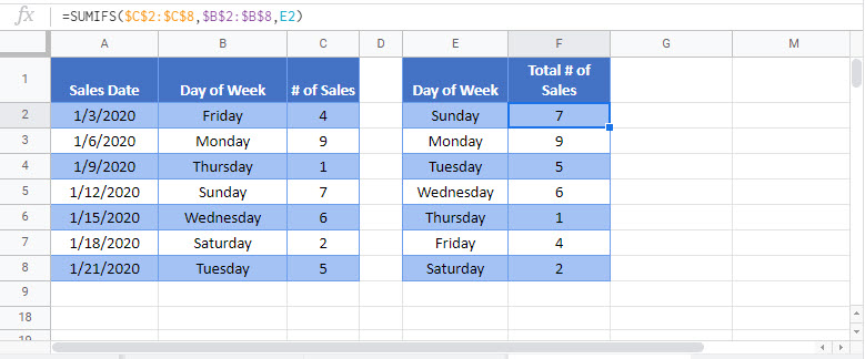
Sum If by Day of Week in Google Sheets
These formulas work exactly the same in Google Sheets as in Excel.
