SUMPRODUCT IF Formula – Excel & Google Sheets

This tutorial will demonstrate how to calculate “sumproduct if”, returning the sum of the products of arrays or ranges based­­ on criteria.

 

SUMPRODUCT Function

The SUMPRODUCT Function is used to multiply arrays of numbers, summing the resultant array.

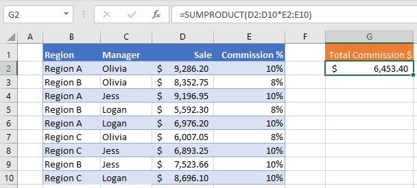
To create a “Sumproduct If”, we will use the SUMPRODUCT Function along with the IF Function in an array formula.

SUMPRODUCT IF

By combining SUMPRODUCT and IF in an array formula, we can essentially create a “SUMPRODUCT IF” that works similar to how the built-in SUMIF function works. Let’s walk through an example.

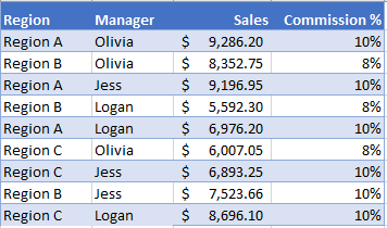
We have a list of sales by mangers in different regions with corresponding commission rates:

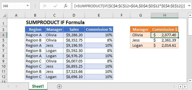
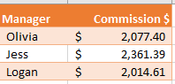
Supposed we are asked to calculate the commission amount for each manager like so:

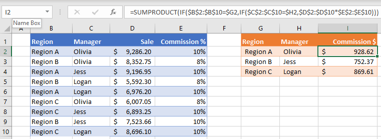
To accomplish this, we can nest an IF function with the manager as our criteria inside of the SUMPRODUCT function like so:

=SUMPRODUCT(IF(<criteria range>=<criteria>,<values range1>*<values range2>))

=SUMPRODUCT(IF($C$2:$C$10=$G2,$D$2:$D$10*$E$2:$E$10))

When using Excel 2019 and earlier, you must enter the formula by pressing CTRL + SHIFT + ENTER to get the curly brackets around the formula (see top image).

How does the formula work?

The formula works by evaluating each cell in our criteria range as TRUE or FALSE.

Calculating the total commission for Olivia:

=SUMPRODUCT(IF($C$2:$C$10=$G2,$D$2:$D$10*$E$2:$E$10))

= SUMPRODUCT (IF({TRUE; TRUE;FALSE; FALSE; FALSE; TRUE; FALSE; FALSE; FALSE}, {928.62; 668.22;919.695; 447.384; 697.620; 480.564; 689.325; 752.366; 869.61}))

Next, the IF Function replaces each value with FALSE if its condition is not met.

= SUMPRODUCT({928.62; 668.22; FALSE; FALSE; FALSE; 480.564; FALSE; FALSE; FALSE})

Now the SUMPRODUCT Function skips the FALSE values and sums the remaining values (2,077.40).

SUMPRODUCT IF with multiple criteria

To use SUMPRODUCT IF with multiple criteria (similar to how the built-in SUMIFS function works), simply nest more IF functions into the SUMPRODUCT function like so:

=SUMPRODUCT(IF(<criteria1 range>=<criteria1>, IF(<criteria2 range>=<criteria2>, <values range1>*<values range2>))

=SUMPRODUCT(IF($B$2:$B$10=$G2,IF($C$2:$C$10=$H2,$D$2:$D$10*$E$2:$E$10)))

(CTRL + SHIFT + ENTER)

Another approach to SUMPRODUCT IF

Often in Excel, there are multiple ways to derive to the desired results. A different way to calculate “sumproduct if” is to include the criteria within the SUMPRODUCT function as an array using double unary like so:

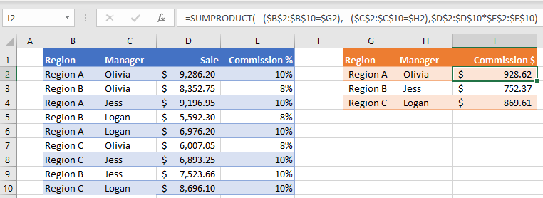
=SUMPRODUCT(--($B$2:$B$10=$G2),--($C$2:$C$10=$H2),$D$2:$D$10*$E$2:$E$10)

This method uses the double unary (–) to convert a TRUE FALSE array to zeros and ones. SUMPRODUCT then multiplies the converted criteria arrays together:

=SUMPRODUCT({1;1;0;0;0;1;0;0;0},{1;0;1;0;1;0;0;0;0},{928.62; 668.22;919.695; 447.384; 697.620; 480.564; 689.325; 752.366; 869.61})

Tips and tricks:

• Where possible, always lock-reference (F4) your ranges and formula inputs to allow auto-filling.
• If you are using Excel 2019 or newer, you may enter the formula without Ctrl + Shift + Enter.

 

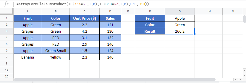
SUMPRODUCT IF in Google Sheets

The SUMPRODUCT IF Function works exactly the same in Google Sheets as in Excel, except you must use the ARRAYFORMULA Function instead of CTRL+SHIFT+ENTER to create the array formula.