VLOOKUP – Display Multiple Matches (Rows of Results)

In this Excel Tutorial you will learn how to deal with multiple matches (results) from a VLOOKUP Function. We will cover two different techniques. The first actually uses the VLOOKUP Function (along with COUNTIF). The second uses INDEX / MATCH to simulate a VLOOKUP.

VLOOKUP with Multiple Results

To lookup multiple matches with the VLOOKUP Function you need to create a helper column within the table of data. The helper column uses the COUNTIF Function to create a unique ID for each instance. The helper column must be the leftmost column within the data set. If it’s not practical to adjust the data set, you should look into the other method in the next section.

Let’s take a look at this method in practice:

Step 1:

Notice the formula in cell F6:
=B5&COUNTIF(B5:B$9,B5)
Specifically, the range referenced: B6:B$11 . Notice the $ Sign. The $ Sign “locks” the cell reference: B$11. So as you copy the formula down, B$11 stays locked. B6, however, is not locked, so as you copy the formula down B6 turns into B7, etc. This technique, creates a unique number for each instance found. The reason we leave B6 unlocked is so that as an instance is accounted for, it’s removed from the total count, creating the unique number.

Also notice the &. & merges the Product Name with it’s instance number to create one field that we will use in our lookup.

Step 2:

We’ve moved the new helper column (project_adj) to the left of the data set in B14:C19. Now we can perform the VLOOKUP on multiple results. Instead of searching for socks, search for socks1 and socks2. Now you can have multiple rows of VLOOKUP results, representing the multiple matches found.

The downside to this method is you must edit the original data set (or copy/paste the data set elsewhere) to perform the multiple results VLOOKUP. Alternatively, you can use INDEX / MATCH Method:

INDEX / MATCH for Multiple Match Lookups

Most Excel users are aware of the power of the VLOOKUP Function, but many are not aware of the power of the INDEX Function and the Match Function used in combination. The INDEX / MATCH combination can be used to emulate a VLOOKUP, with the advantage of more flexibility.

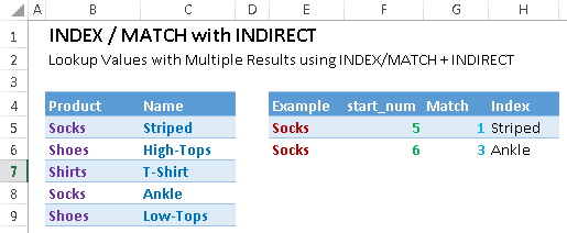
Note: The image directly below contains the formulas. The bottom image contains the formula results.

What’s going on in the formulas above?

MATCH – Looks up a value’s position with a range. In this example, MATCH is searching for “Socks” within the Product list.
INDIRECT – Creates a reference from a string of text. We use this to adjust the Product list search array. Once a match is found, the range is adjusted to exclude that match from the search, allowing the next match to be found. In cell G5, we set the initial range to B5:B10 (by setting the initial start_num in cell F5 to 5). In G5 we found a match in row 1 of the range, so F6’s start_num is 5+1=6.
INDEX – Returns a value from an array based on it’s column/row number position in that array.

!!I guess include the array formula so they have 1 formula to link…