VLOOKUP Duplicate Values – Excel & Google Sheets
Download the example workbook
This tutorial will demonstrate how to lookup duplicate values using VLOOKUP in Excel and Google Sheets. If your version of Excel supports XLOOKUP, we recommend using XLOOKUP instead as this allows for a much easier solution..

VLOOKUP Nth Match
The VLOOKUP Function always returns the first match. In order to return duplicate values (or the nth match) we need:
- A new unique identifier to differentiate all duplicate values.
- A helper column containing a list of unique IDs that will serve as the new lookup column (first column) of the table array.
- A modified lookup value to match the format of the unique IDs.
This is how the final solution will look like:
=VLOOKUP(F3&"-"&G3,B3:D7,3,FALSE)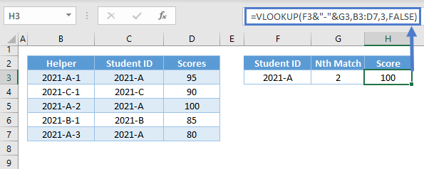
Now, let’s walk through the solution:
Unique IDs using COUNTIF
Let’s say we want to lookup the second score for Student ID = 2021-A in this dataset:

First, we will create unique IDs in column B by joining the original student ID (column C) with a COUNTIF Function:
=C3&"-"&COUNTIF($C$3:C3,C3)
The COUNTIF Function counts the number of each Student ID. By locking one cell reference in the COUNTIF Function, but not the other, we identify each instance of a duplicate Student ID with a unique number:
=COUNTIF($C$3:C3,C3)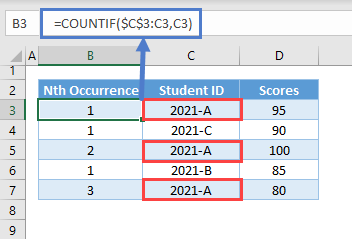
Then we simply use the & operate to concatenate everything together as in the previous formula.
VLOOKUP Nth Match
Now, we can VLOOKUP the 2nd match using this formula where the lookup value matches the format of the new Unique ID:
=VLOOKUP(F3&"-"&G3,B3:D7,3,FALSE)
VLOOKUP All Matches
Instead, what if you want to lookup all matches?
You could manually list out each match that you want to find:
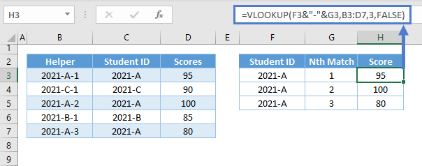
This might be an acceptable solution, but what if you don’t know how many matches exist? This formula will output all matches for “2021-A”:
=IFNA(VLOOKUP($F$2&"-"&ROW(1:1),$B$3:$D$7,3,FALSE),"")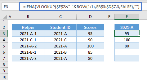
Let’s walk through the formula above:
ROW Function
We use the ROW Function to return the row number of a cell or a range. If we want a formula that can create a list of consecutive counting numbers starting from 1, we can input a whole row reference in the ROW Function and copy and paste it down the column.
=ROW(1:1)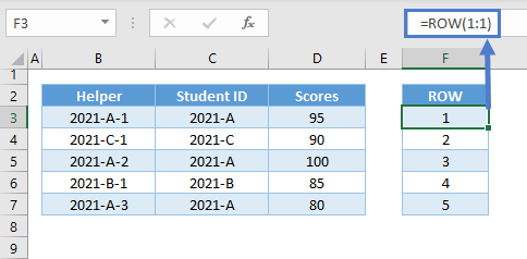
New Lookup Value
Next, use the result of the ROW Function is combined with the lookup value (Column G Header) to create your unique lookup value.
=$G$2&"-"&F3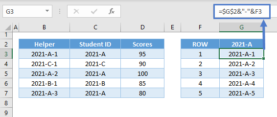
Note: Make sure that the original lookup value is in absolute reference (e.g., $G$2).
VLOOKUP Function
Next, perform the VLOOKUP:
=VLOOKUP(G3,$B$3:$D$7,3,FALSE)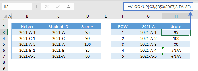
IFNA Function
Notice the #N/A errors for values that don’t exist. Next, let’s use the IFNA Function to output blank instead:
=IFNA(H3,"")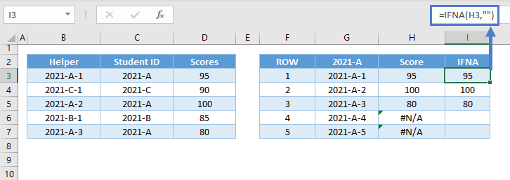
Combining all functions results to our original formula:
=IFNA(VLOOKUP($F$2&"-"&ROW(1:1),$B$3:$D$7,3,FALSE),"")
There’s a more convenient and simpler solution than the formula above, and that is by using the new FILTER Function. We can use the FILTER Function to filter the data and extract the duplicates in one go, but this function is currently only available to Microsoft 365 version. If you have Microsoft 365, then you should use the XLOOKUP Function instead.
VLOOKUP Duplicate Lookup Values
Now, what if we want to match duplicate lookup values to their corresponding instances from the lookup column?
In this case, we apply the same method from the previous sections to the lookup value:
=VLOOKUP(F3&"-"&COUNTIF($F$3:F3,F3),$B$3:$D$7,3,FALSE)
VLOOKUP nth Match in Google Sheets
All VLOOKUP formulas that we have discussed above work the same way in Google Sheets.
=VLOOKUP(F3&"-"&G3,B3:D7,3,FALSE)