HYPERLINK Formula – Clickable Link – Excel, VBA, & G Sheets
Download the example workbook
This Tutorial demonstrates how to use the Excel HYPERLINK Function in Excel to create a clickable link.
HYPERLINK Function Overview
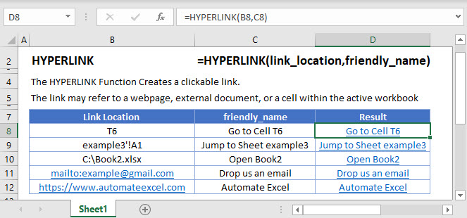
The HYPERLINK Function Creates a clickable link. The link may refer to a webpage, external document, or a cell within the active workbook.
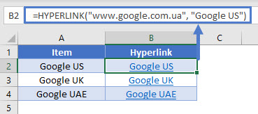
To use the HYPERLINK Excel Worksheet Function, select a cell and type:
![]()
(Notice how the formula inputs appear)
HYPERLINK Function Syntax and Inputs:
=HYPERLINK(link_location,friendly_name)link_location – The file path, web address, or link address. Example: “www.excelbootcamp.com”
friendly_name – The link name to display. Example: Excel Boot Camp
HYPERLINK Function
The HYPERLINK Function creates a clickable shortcut which redirects users from one location to another. The location can be a cell/sheet in a workbook, another workbook, email address, file on the internet or a network server.
Once the hyperlink is created, the clickable shortcut or [friendly_name] is the text that displays instead of the entire URL.
HYPERLINK Function – Cell Reference
The HYPERLINK Function can jump to a cell reference within the same workbook.
=HYPERLINK("#T6", "Go to Cell T6")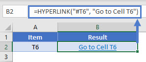
HYPERLINK Function – Sheet Reference
Similarly the HYPERLINK Function can also jump to a sheet reference within the same workbook.
=HYPERLINK("#'example3'!A1","Jump to Sheet example3")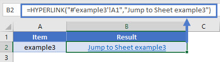
HYPERLINK Function – File Location
Absolute Path
The HYPERLINK Function can open a different workbook or any file present on your system.
=HYPERLINK("X:\Book2.xlsx","Open Book2")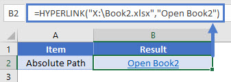
Note: the hyperlink will not work if you change file location
Relative Path
In case the file location is expected to change, we can use a relative path in the HYPERLINK Function.
=HYPERLINK("Excel files\Book3.xlsx","Open Book3")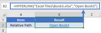
HYPERLINK Function – Email Address
The HYPERLINK Function can send a message to a specific recipient.
=HYPERLINK("mailto:example@gmail.com","Drop us an email")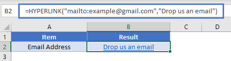
HYPERLINK Function – Webpage
The HYPERLINK Function can redirect users to a specific webpage.
=HYPERLINK("https://learn.autovbax.com/","Learing VBA")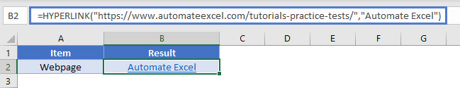
HYPERLINK, INDEX & MATCH Function
The HYPERLINK Function can be used with INDEX & MATCH Function to create hyperlinks that pull a matching value & create a shortcut to it.
=HYPERLINK("#"&CELL("address", INDEX(A2:A6, MATCH(D2, B2:B6,0))), INDEX(A2:A6, MATCH(D2, B2:B6,0)))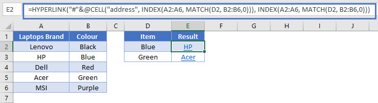
Multiple HYPERLINKS
When using the HYPERLINK Function, multiple hyperlinks can be edited at the same time. Open the Find & Replace dialogue by pressing Ctrl+H.
- In the dialogue, enter the old link in Find what: box & new link in the Replace with: box.
- Click the Look in: dropdown and select Formulas.
- Now click Replace All button
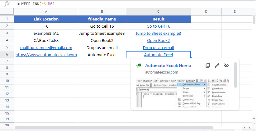
HYPERLINK in Google Sheets
The HYPERLINK Function works exactly the same in Google Sheets as in Excel:
Additional Notes
Use the HYPERLINK Function to create a hyperlink to a cell within the workbook, an external file, or a webpage. Clicking the link will “goto” to reference. Depending on the type of hyperlink, this may open a web browser, another file, or simply jump to the referenced cell in the activate workbook.
To select a cell containing a hyperlink, without opening it, select the cell using the arrow keys.
If you use the hyperlinks that open webpages in Excel you may want to change the text that identifies the link(called Anchor text in webspeak).
Usually you can just type a URL in a cell and it automatically converts to a Hyperlink. This works fine for linking to Domains, however when I link to individual pages the link looks long and ugly. Fortunately Excel provides a way to choose the text that displays. Excel calls it friendly_name.
To control the text that displays for a Hyperlinked cell, enter your link as follows:
Syntax
=HYPERLINK(link_location,[friendly_name])
Example
=HYPERLINK(“https://www.autovbax.com”,”Automate AutoVBA Home Page”)