IFS Function Examples – Excel & Google Sheets

This tutorial demonstrates how to use the IFS Function in Excel and Google Sheets.

IFS Function Overview

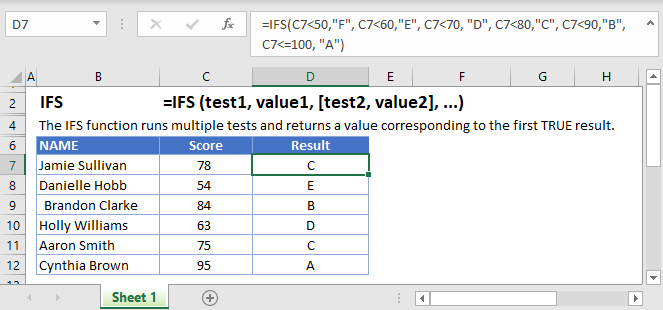
The Excel IFS function runs multiple tests and returns a value corresponding to the first TRUE result.

To use the IFS Excel Worksheet Function, select a cell and type:

(Notice how the formula inputs appear)

IFS function Syntax and inputs:

=IFS (test1, value1, [test2, value2], ...)

test1 – First logical test.

value1 – Result when test1 is TRUE.

test2, value2 – [optional] Second test/value pair.

 

What is the IFS Function?

IFS is a “conditional” function. You define a series of logical tests, each with a return value associated with it. Excel works through each of your tests in turn, and as soon as it finds one that evaluates to TRUE, it returns the value you associated with that test.

This works much the same was as when nesting multiple IF statements, but tends to be easier to read and work with.

How to Use the IFS Function

You use the Excel IFS Function like this:

=IFS(C3<50,"F", C3<60,"E", C3<70, "D", C3<80,"C", C3<90,"B", C3<=100, "A")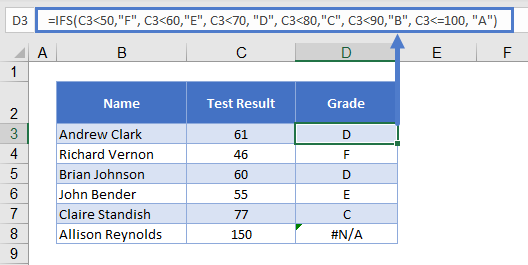

This formula takes a student’s test score, and converts it into their grade for that test.

The formula may look complicated, but it makes more sense if you put each test on a separate line:

=IFS(
C3<50,"F",
C3<60,"E",
C3<70, "D",
C3<80,"C",
C3<90,"B",
C3<=100, "A"
)

That’s better! It’s much clearer now that we have a series of tests paired with a return value. Excel works down the list until it gets a match, and then returns the grade that we’ve paired with that score.

You can define up to 127 tests in the IFS Function.

Setting a Default Value

With the normal IF statement, we define two values that Excel can return: one for when the logical test is true, and another for when it is false.

IFS doesn’t have the option to add a false return value, and if Excel doesn’t find a match in any of your tests, it will return #N/A. Not good. But, we can get around this by setting a default value.

It works like this:

=IFS(
C3<50,"F",
C3<60,"E",
C3<70, "D",
C3<80,"C",
C3<90,"B",
C3<=100, "A"
TRUE, “Unknown”
)

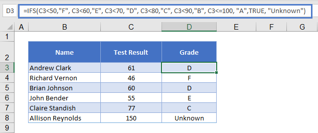
We’ve set up a final logical test – just “TRUE”, by itself.

TRUE, naturally, evaluates to TRUE. So, if Excel doesn’t find a match in our previous tests, the final test will always be triggered, and Excel will return “Unknown.”

 

What IFS can return

Above we told IFS to return a text string – the grade associated with each test score. But you can also return numbers, or even other formulas.

For example, if you have a sales team, and you pay them commission based on the value of each sale, you could use IFS to calculate their commission according to the sale value.

=IFS(
C3<20000,C3*0.02,
C3<40000,C3*0.03,
C3<60000, C3*0.04,
C3 >=60000, C3*0.05,
TRUE, 0
)

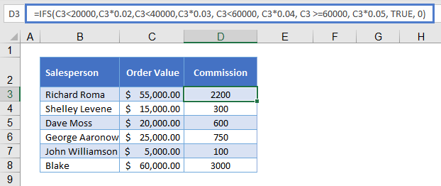
Now IFS will check the value in C3, and then return the associated formula when it finds a match. So sales below $20,000 earn 2% interest, below $40,000 earns 3%, and so on.

For good measure, we’ve also set a default value of 0.

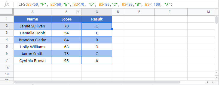
IFS in Google Sheets

The IFS Function works exactly the same in Google Sheets as in Excel: