INDIRECT Fx – Cell Reference from Text – Excel & G Sheets

This Tutorial demonstrates how to use the Excel INDIRECT Function in Excel to create a cell reference from text.

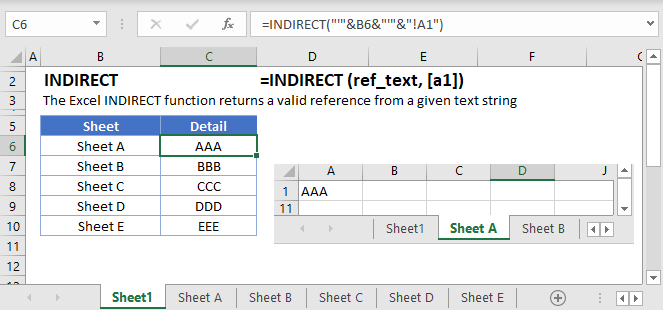
INDIRECT Function Overview

The INDIRECT Function Creates a cell reference from a text string.

(Notice how the formula inputs appear)

INDIRECT function Syntax and inputs:

=INDIRECT(ref_text,C1)

ref_text – A string representing a cell reference or range reference. The string can be in R1C1 or A1 format, or can be a named range.

a1 – OPTIONAL: Indicates whether the reference is in R1C1 or A1 format. FALSE for R1C1 or TRUE / Ommitted for A1.

What is the INDIRECT function?

The INDIRECT function allows you to give a text string and have the computer interpret that string as an actual reference. This can be used to reference a range on the same sheet, a different sheet, or even a different workbook.

CAUTION: The INDIRECT function is one of the volatile functions. Most of the time when you’re working in your spreadsheet, the computer will only recalculate a formula if the inputs have changed their values. A volatile function, however, recalculates every time you make a change to any cell. Caution should be used to ensure that you don’t cause a large recalculation time due to excessive use of volatile function or having many cells dependent upon the result of a volatile function.

Create a cell reference

Say that you want to fetch the value from A2, but you want to make sure that your formula stays on A2 regardless of new rows being inserted/removed. You could write a formula of

=INDIRECT("A2")

Note that the argument inside our function is the text string “A2”, and not a cell reference. Also, since this is a text string, there’s no need to indicate an absolute reference like $A$2. The text will never change, and thus this formula will always point to A2, no matter where it gets moved to.

INDIRECT row number

You can concatenate text strings and values from cells together. Rather than writing “A2” like we did previously, we can grab a numerical value from cell B2 and use that in our formula. We would write out formula like

=INDIRECT("A" & B2)

The “&” symbol is being used here to concatenate the text string “A” with the value from cell B2. So, if the value of B2 was currently 10, then our formula would read this as

=INDIRECT("A" & 10)
=INDIRECT("A10")
=A10

INDIRECT column value

You can also concatenate in the column reference. This time let’s say that we know we want to grab a value from row 10, but we want to be able to change what column to pull from. We’ll put the column letter we want in cell B2. Our formula could look like

=INDIRECT(B2 & "10")

If the value of B2 is “G”, then our formula evaluates like so

=INDIRECT("G" & 10)
=INDIRECT("G10")
=G10

INDIRECT r1c1 style

In our previous example, we had to use a letter to indicate column reference. This is because we were using what’s known as A1 style referencing. In A1 style, columns are given by a letter, and rows are given by numbers. Absolute references are indicated using the “$” before the item we want to remain absolute.

In r1c1, both rows and columns are started using number. The absolute reference to a1 would be written as

=R1C1

You can read this as “Row 1, Column 1”. Relative references are given by using brackets, but the number indicates position relative to cell with formula. So, if we were writing a formula in cell A10 and we need to refer to A1, we’d write the formula

=R[-9]C

You can read this as “The cell 9 rows up, but in the same column.

The reason this might be helpful is that INDIRECT can support the use of r1c1 notation. Consider the previous example where we were fetching a value from row 10 but wanted to be able to change the column. Rather than giving a letter, let’s say that we put a number in cell B2. Our formula then might look like

=INDIRECT("R10C" & B2, FALSE)

We’ve been omitting the 2^nd argument up till now. If this argument is omitted or True, the function will evaluate using A1 style. Since it’s False, it’s going to evaluate in r1c1. Let’s assume the value of B2 is 5. Our formula will evaluate this like so

=INDIRECT("R10C5", FALSE)
=$E$10

INDIRECT differences with A1 vs r1c1

Remember that we previous showed that since the contents of this formula was a text string, it never changed?

=INDIRECT("A2")

This formula will always be looking at cell A2, no matter where you move the formula. In r1c1, since you can indicate relative position using brackets, this rule doesn’t stay consistent. If you place this formula in cell B2

=INDIRECT("RC[-1]")

It will be looking at cell A2 (since column A is one to the left of column B). If you copy this formula to cell B3, the text inside will remain the same, but the INDIRECT will now be looking at cell A3.

INDIRECT with sheet name

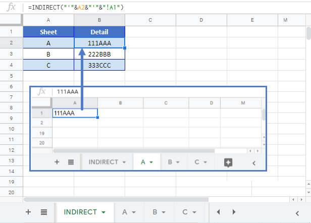
You can also combine a sheet name into your INDIRECT references. An important rule to remember is that you should place single quotation marks around the names, and you need to separate the sheet name from the cell reference with an exclamation mark.

Let’s say we had this setup, where we are stating our sheet name, row, and column.

Our formula to combine all of these into a reference would look like this:

=INDIRECT("'" & A2 & "'!" & B2 & C2)

Our formula will then get evaluated like so:

=INDIRECT("'" & "Sheet2" & "'!" & "B" & "5")
=INDIRECT("'"Sheet2'!B5")
='Sheet2'!B5

Technically, since the word “Sheet2” doesn’t have any spaces in it, we don’t need the single quotation marks. It’s perfectly valid to write something like

=Sheet2!A2

However, it doesn’t hurt to place the quotation marks when you don’t need them. It’s best practice to include them so that your formula can handle instance where they might be needed.

INDIRECT to another workbook

We will also mention that INDIRECT can create a reference to a different workbook. The limitation is that INDIRECT won’t fetch values from a closed workbook, so this particular use has limited practicality. If the workbook that INDIRECT is pointing to is unopened, the function will throw a “#REF!” error.

The syntax when writing the workbook name is that it needs to be in square brackets. Let’s use this setup and try to fetch a value from cell C7.

Our formula would be

=INDIRECT("'[" & A2 & "]" & B2 & "'!C7")

Again, pay attention to the placement of the single quotation marks, brackets, and exclamation mark. Our formula will then get evaluated like so:

=INDIRECT("'[" & "Sample.xlsx" & "]" & "Summary" & "'!C7")
=INDIRECT("'[Sample.xslx]Summary'!C7")
='[Sample.xlsx]Summary'!C7

INDIRECT to build dynamic range

When you have a large data set, it’s important to try and optimize the formulas so that they aren’t doing more work than needed. For instance, rather than referencing all of column A, we might want to just reference the exact number of cells in our list. Consider the following layout:

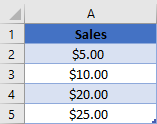
In cell B2, we’ve placed the formula

=COUNTA(A:A)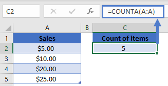

The COUNTA function is very easy for the computer to calculate, as it simply checks how many cells in col A have some value, as opposed to having to do any logic checks or mathematical operations.

Now, let’s build our formula that will sum the values in column A, but we want to make sure it only looks at the exact range with values (A2:A5). We will write our formula as

=SUM(INDIRECT("A2:A" & B2))

Our INDIRECT is going to grab the number 5 from cell B2 and will create a reference to the range A2:A5. The SUM can then use this range for its calculation. If we add another value into cell A6, then the number in B2 will update, and our SUM formula will auto-update as well to include this new value.

CAUTION: With the introduction of Tables in Office 2007, it’s much more efficient to store your data in a table and use a structural reference rather than build the formula we used in this example due to the volatile nature of INDIRECT. However, they may be instances where you need to create a list of items and can’t use a Table.

Dynamic Charting with INDIRECT

Let’s take the previous example and go one more step. Rather than writing a formula to give us the sum of the values, we’ll create a Named Range. We could call this range “MyData” and have it refer to

=INDIRECT("A2:A" & COUNTA($A:$A))

Note that since we’re putting this in a Named Range, we’ve swapped the reference to B2 and instead put the COUNTA function in there directly.

Now that we have this named range, we could use it in a chart. We’ll create a blank line chart, and then add a data series. For the series values, you could write something like

=Sheet1!MyData

The chart is now going to be using this reference to plot values. As more values are added to column A, the INDIRECT will refer to a larger and larger range, and our chart will continue to stay updated with all the newly added values.

Dynamic Data Validation with INDIRECT

When gathering input from users, sometimes there is a need to make one choice’s options to choose from dependent upon a previous choice. Consider this layout, where our first column allows user to choose between Fruits, Vegetables, and Meats.

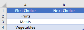
In the 2^nd column, we don’t want to have a large list showing every possible choice, as we’ve already narrowed things down a little bit. So, we’ve created 3 other lists that look like this:

Next, we’ll assign each of these lists to a Named Range. I.e., all the fruits will be in a range called “Fruits”, and vegetables in “Vegetables”, etc.

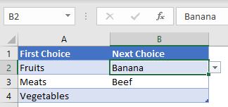
Back in our table, we’re ready to setup the data validation in the 2^nd column. We’ll create a List type validation, with an input of:

=INDIRECT(A2)

The INDIRECT is going to read in the choice made in col A and see the name of a category. We’ve defined ranges with these names, so the INDIRECT will then take that name and create a reference to the desired range.

Additional Notes

Use the INDIRECT Function to create a cell reference from text.

First create the string of text that represents a cell reference. The string must either be in the usual A1-Style column letter & row number (M37) or in R1C1-style (R37C13). You can type the refernce directly, but usually you will reference cells which define the rows and columns. Last, enter which cell reference format you choose. TRUE or Omitted for A1-Style reference or FALSE for R1C1-style.

While working with INDIRECT Formulas, you may want to use the ROW Function to get the row number of a reference or the COLUMN Function to get the column number (not letter) of a reference.

INDIRECT in Google Sheets

The INDIRECT Function works exactly the same in Google Sheets as in Excel: