LARGE Function Examples in Excel, VBA, & Google Sheets

This tutorial demonstrates how to use the Excel LARGE Function in Excel to calculate the nth largest value.

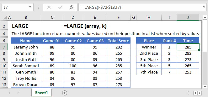
LARGE Function Overview

The LARGE Function Calculates the kth largest value.

To use the LARGE Excel Worksheet Function, select a cell and type:

(Notice how the formula inputs appear)

LARGE function Syntax and inputs:

=LARGE(array,k)

array – An array of numbers.

k – The position of the value you want to return. Example: 6 would return the 6th largest value.

 

How to use the LARGE Function

The LARGE Function returns the k-th largest number from a range of values. It is the opposite of the SMALL Function. 

To use the LARGE function, use the following formula:

=LARGE(B2:B9, 3)

Here we are looking for the 3rd largest number (3rd oldest student) in the range B2:B9.

Out of Range Error

If you enter a number k, greater than the number of items in the range, the LARGE Function will return #NUM! error

=LARGE(B2:B8, 8)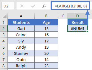

Notice here we are looking for the 8th largest number in a range of only 7 numbers. So the LARGE Function returns #NUM!.

Non-numeric Data

The LARGE Function will completely ignore non-numeric data as if that data is not part of the data range.

=LARGE(B2:B8, 4)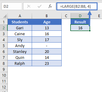

LARGE If

We can use the LARGE Function with criteria as well to perform a “large if”. For example, let’s say we want to find the 2nd oldest male student.

We will use this array formula:

{=LARGE(IF(B2:B8 = "M", C2:C8), 2)}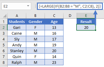

Note: When building array functions, you must press CTRL + SHIFT + ENTER instead of just ENTER after creating your formula.

You’ll notice how the curly brackets appear. You can not just manually type in the curly brackets; you must use CTRL + SHIFT + ENTER.

To learn more about how the LARGE “IF” formula works, read our tutorial on LARGE If and LARGE IF.

Sort with the LARGE Function

A quite useful use case for the LARGE Function is to sort data in descending (largest to smallest) order. To sort data, we combine the LARGE function with the ROW function.

=LARGE($A$2:$A$8, ROW()-1)

This function works by using the ROW Function to define the k-value. Notice how row 2 has the largest number (k = 1), row 3 has the second largest (k = 2), so on & so forth. Thus, sorting the range from largest to smallest.

To learn more read our tutorial on Sorting with the SMALL and LARGE Functions.

Note: The above formula uses absolute references (the $ signs) to lock cell references when copying formulas. If you aren’t familiar with this, please read our Excel References Guide (link to: https://learn.autovbax.com/basics/cell-references.html  )

 

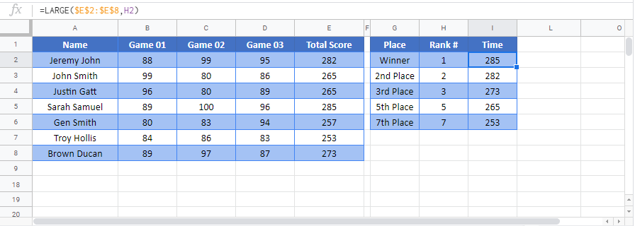
LARGE function in Google Sheets

The LARGE function works exactly the same in Google Sheets as in Excel.

LARGE Examples in VBA

You can also use the LARGE function in VBA. Type:
application.worksheetfunction.large(array,k)
For the function arguments (array, etc.), you can either enter them directly into the function, or define variables to use instead.