MATCH Worksheet Function in Excel, VBA, & Google Sheets
Download the example workbook
This tutorial demonstrates how to use the MATCH Function in Excel, VBA, and Google Sheets to find a value.
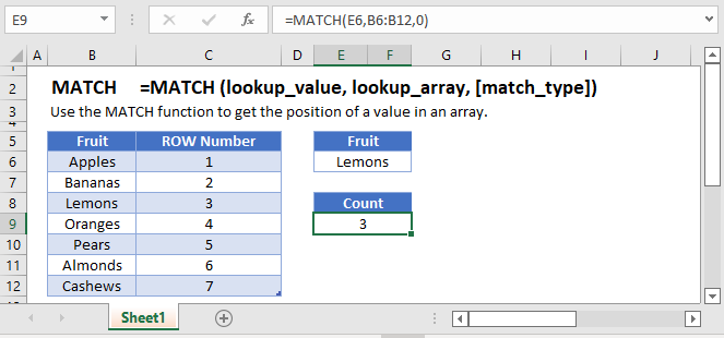
What is the MATCH function?
The MATCH Function Searches for an item in a list and returns a number representing it’s position in the list.
It is often used in conjunction with the INDEX Function to create a lookup formula (similar to VLOOKUP or XLOOKUP). This tutorial will cover these use-cases and more.
MATCH Function – Exact Match
You will often come across large lists of data and you need to be able to search for a specific item. We’ll use a small example with some fruit. First, we’ll look for an exact match. Here’s the layout of our data. We want to search for the word in cell D1.
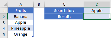
In D2, our formula is:
=MATCH(D1, A2:A5, 0)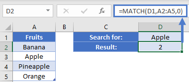 Take note that we needed to specify either 0 or False as the last argument to indicate that we want an exact match. The result from this function is 2, because “Apple” is the 2nd item in our range.
Sorted list
Let’s see how the MATCH function works with a non-exact match. Here we have a list of items. NOTE: The items have been sorted in ascending order.
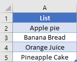
In D1, we’ve said that we want to look for the word “Orange”. The formula in D2 is
=MATCH(D1, A2:A5, 1)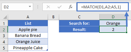 Our formula gives a result of 2 even though “Orange Juice” is in the 3rd cell. Because we were searching for a closest match, the function will find either our exact word, or the next smallest item. With text strings, this happens to be the word just before “Orange Juice”, and so we got a result of 2.
This ability to find next smallest may be easier to understand using a number search. Consider this layout, where we’ve only listed items by 10. If we search for a value of 34 using our formula, you can see that the result is 3.
=MATCH(D1, A2:A5, 1)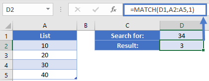
This can work well when you are dealing with “buckets”, and you just want to be able to find out which group a value belongs in.
Descending list
In our previous example, what if you wanted the value of 34 to be placed in the larger group? In our next example, let’s say that we have a list of difference sized shipping containers and we need to know which one to use. Since we need to make sure we have enough room or more, we’ll use the MATCH function with the last argument set to -1. Let’s look at this example:
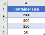
In this case, we need to find out which container will fit our size of 495. The formula in D2 is:
=MATCH(D1, A1:A5, -1)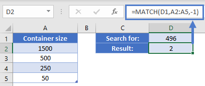 The result of this formula is 2, indicating that we need to use the 2nd item from the list (the 500) to fit our needs.
Wildcard match
The MATCH Function also supports the use of wildcards like “*” and “?”. Let’s go back to our list of various food items. In this case, we’ve changed our search term in D1 to be “Orange*”.

Our formula in D2 is:
=MATCH(D1, A1:A5, 0)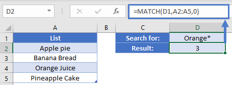 Note that we need to switch the MATCH type back to exact match. Even though the items are mixed up and our search term did not have the full text match, our formula was able to give the correct result of 3.
Using MATCH with INDEX
Returning the relative position of an item is nice, but it’s usually not that helpful to human users. We usually want to know the corresponding value for an item. This is where INDEX can enter the scene. As INDEX needs a numerical position for row and/or column, we can use the MATCH function to tell the INDEX which item we want. Consider the following layout where we need to be able to lookup prices for our items.

We are searching for “Apple”. In E2, our formula is
=INDEX(A2:A5, MATCH(E1, B2:B5, 0))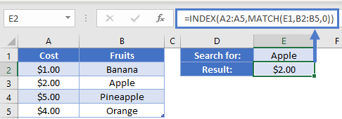
The MATCH function is going to search B2:B5 for our exact phrase, “Apple”. It will find this in the 2nd item and return the value of 2. The INDEX then takes this and will give us the 2nd value from the A2:A5 range. The 2nd item is in cell A3, the $2.00.
Match in Google Sheets
The MATCH Function works exactly the same in Google Sheets as in Excel:

MATCH Examples in VBA
You can also use the MATCH function in VBA. Type:
application.worksheetfunction.match(lookup_value,lookup_array,match_type)
For the function arguments (lookup_value, etc.), you can either enter them directly into the function, or define variables to use instead.
Assuming we have the following values in our Excel sheet

executing the following code
Dim Match_Value  As Variant
Match_Value = Application.WorksheetFunction.Match("test1", Range("A4:A13"), 1)
MsgBox ("Match was found at row  " & Max_Value)
Will return the following
Match was found at row 9because the string “test1” is the ninth element in the range of values to be searched.
We can also search for content in our worksheet instead of directly entering values in the VBA code: The following statement will search Column A for the whatever value is entered in cell C3
Match_Value = Application.Match(Cells(3, 3).Value, Columns(1), 0)