How to use the TREND Function – Excel, VBA, Google Sheets

This tutorial demonstrates how to use the Excel TREND Function in Excel to calculate y-values based on a trendline.

TREND Function Overview

The TREND Function Calculates Y values based on a trendline for given X values. The trendline is calculated Using the least squares method based on two data series.

To use the TREND Excel Worksheet Function, select a cell and type:

(Notice how the formula inputs appear)

TREND function Syntax and inputs:

=TREND(known_ys,known_xs,new_xs,const)

known_y’s – An array of known Y values.

known_x’s – An array of known X values.

new_x’s – An array of new X values that you want TREND to return corresponding Y values for.

const – OPTIONAL. Logical value indicating whether to calculate B (the intercept in y = mx + b) using the least squares method (TRUE Or Ommitted) or to manually set B = 0 (FALSE).

What is TREND?

The TREND function in Excel is like the FORECAST function, used to predict an x value given known x and y values, except that it applies the regression equation for an array of x values. The function uses linear regression to determine the result. It is recommended to visit the FORECAST function [insert link to FORECAST page] before viewing this page to learn about linear regression.

How to use TREND

The TREND function takes four arguments:

=TREND(known_y’s, known_x’s, new_x’s, const)

Where, known_y’s and known_x’s refer to the x and y data in your data table, new_x’s is an array of data points you wish to predict the y-value for and const is a binary argument for calculating the y-intercept normally, or forcing the value to 0 and adjusting the slope values so that .

Although the latter 3 arguments of TREND are optional, it is recommended to include all arguments to ensure the data prediction is correct.

Let’s look at an example:

=TREND(C3:C7,B3;B7,B10:B17,TRUE)

Using TREND in Microsoft 365 (namely, the Office Insider Current Channel (Preview)), TREND acts as a dynamic array formula which spills the result for the entire array, as shown with the light blue border around cells C10 to C17 in this example. Simply type the formula in cell C10 and hit enter, no need to fill or drag the formula down.

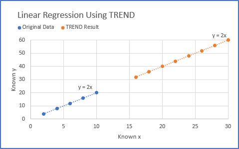
To show the regression equation that TREND found to predict our array of results, I’ve plotted the data:

The equation matches!

Non-Linear Regression with TREND

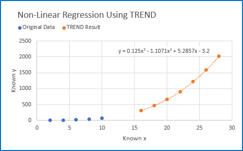
TREND can also be used for polynomial curve fitting.

Adding additional x columns and raising them to the n^th degree fits a polynomial curve to the same degree. All x columns must be included in the arguments for known_x’s and new_x’s.

Graphing it:

TREND TIPS

1. Ensure you have the most updated version of Microsoft 365 to utilize TREND with dynamic arrays. You may need to enable the Office Insider Current Channel (Preview) to utilize dynamic array functions. On the Account Page:

(Not required to use the function, just for dynamic array functionality)

2. If your data is formatted as an Excel table (usually by Ctrl+T), TREND will result in errors. Spilled array formulas are not supported inside of Excel tables. Move your data out of the table and try again.

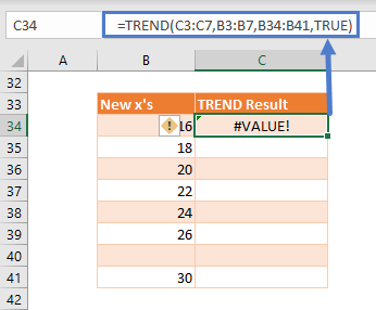
3. If your new x’s array is not full, you will get a #VALUE! Error. Change the range in the function argument so it is continuous.

Interested in More Forecasting?

See our other articles on Forecasting with Exponential Smoothing, LINEST and LOGEST functions.

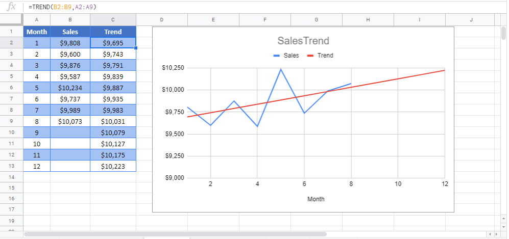
TREND function in Google Sheets

The TREND function works exactly the same in Google Sheets as in Excel.

TREND Examples in VBA

You can also use the TREND function in VBA. Type:
application.worksheetfunction.trend(known_ys,known_xs,new_xs,const)
For the function arguments (known_y’s, etc.), you can either enter them directly into the function, or define variables to use instead.