Use Conditional Formatting With Checkbox in Excel & Google Sheets
This tutorial demonstrates how to use conditional formatting with a checkbox control in Excel and Google Sheets.
Conditional Formatting With Checkbox
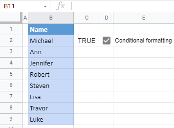
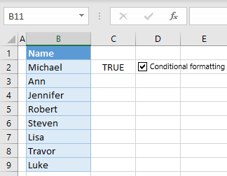
In Excel, you can use a checkbox to control whether or not conditional formatting should be applied. For the following example, you have the data below in Column B and a checkbox linked to cell C2. (Here, we’re starting with an existing checkbox. If there isn’t already one in your worksheet, you’ll need to insert a linked checkbox before you start.)
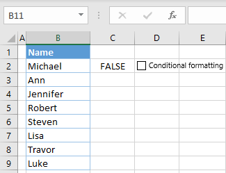
Say you want to create conditional formatting rules for the range (B2: B9) that adds a fill color to the cells when the checkbox is checked. Since the checkbox is linked to cell C2, this cell will have the value TRUE if the checkbox is checked, and FALSE if it’s unchecked. You’ll use the value of cell C2 as the determinant for the conditional formatting rule.
- Select the data range and in the Ribbon, go to Home > Conditional Formatting > New Rule.
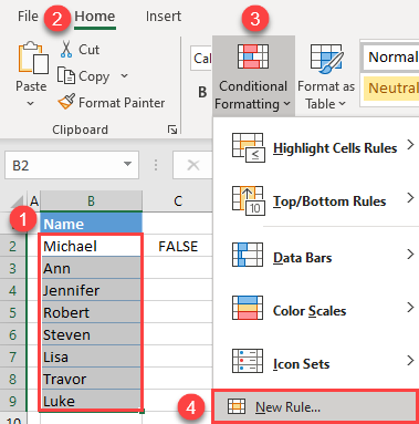
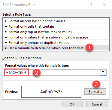
- In the Rule Type menu, (1) select Use a formula to determine which cells to format. This gives you a formula box under Edit the Rule Description. (2) In the box, enter:
=$C$2 = TRUEThen (3) click Format.
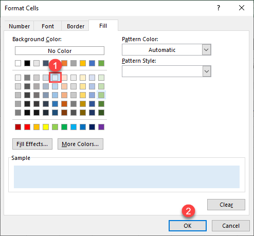
- In the Format Cells window, (1) select a color (e.g., light blue) and (2) click OK.
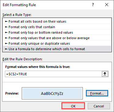
- That takes you back to the Edit Rules window. Click OK.
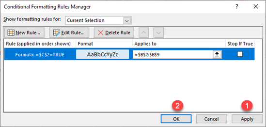
- Click Apply, then OK to confirm the new rule.
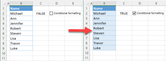
Now, when you check the checkbox, the value of cell C2 becomes TRUE, and all cells in the range (B2:B9) get the light blue background color.
Conditional Formatting With Checkbox in Google Sheets
The process is similar in Google Sheets.
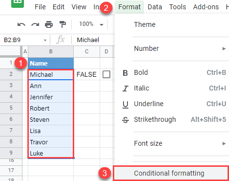
- Select the data range and in the Menu, go to Format > Conditional formatting.
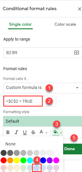
- In the Conditional format rule window on the right, (1) select Custom formula is and (2) enter the formula:
=$C$2 = TRUEFor the Formatting style, (3) select Fill color, (4) choose the background color (i.e., light blue), and (5) click Done.
The result is the same as in the previous example. When the checkbox is checked, cells in B2:B9 are filled with a light blue background.