Set Up Automatic Currency Conversion in Excel & Google Sheets

This tutorial will demonstrate how to create and automatic currency converter in Excel and Google Sheets.

 

 

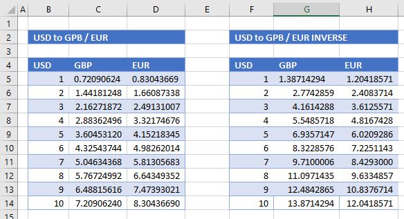
Excel is a powerful tool for calculations, often involving international currencies. Excel does not have a built-in currency conversion tool, but with a link to an external XML database, we can build our own conversion tool into Excel using Power Query.

Linking to an External XML Source File

The most user-friendly source file is one called Floatrates, a free XML feed that is updated daily.

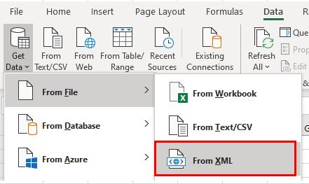
1. In a blank Excel worksheet, in the Ribbon, select Data > Get Data > From File > From XML.

 

 

2. In the File name box type the URL for the floatrates file – www.floatrates.com/daily.usd.xml – and then click Open.

 

 

3. Click on Transform Data.

 

 

4. The Power Query Editor will now open. Scroll across to the last item on the list, and then click on the word Table. The exchange rates will be populated in a table below the initial line of data.

 

 

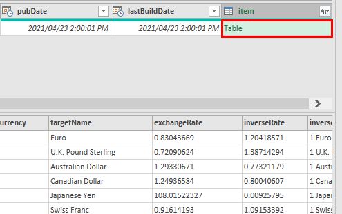
5. Click on the double-headed arrow to show the fields of this table, and then click OK.

 

 

6. The Power Query will now change to show the exchange rate columns as well as the initial columns.

 

 

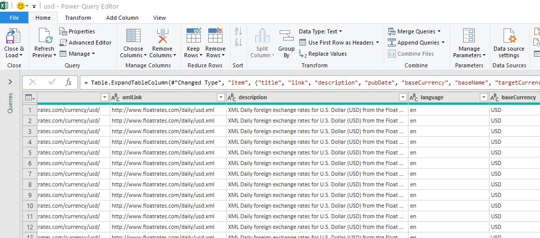
7. In the Ribbon, select Home > Manage Columns > Choose Columns.

 

 

8. Uncheck the columns that are not required, and then click OK.

 

 

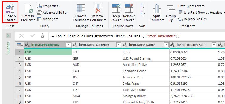
9. Click Close & Load to return to Excel.

 

 

Creating a Currency Converter

1. We can now create a new worksheet in the same workbook as the linked XML database and set up a table as shown below.

 

 

2. We can now use the VLOOKUP Function to look up the currency rate for the British Pound against the US Dollar. In the relevant cell (for example C5), we can type in the following:

=VLOOKUP($C$4,

TIP: Use an absolute reference ($) so we can copy the formula down.

3. We then need to highlight the relevant lookup data by going to the data sheet and selecting the information we require.

 

 

4. As soon as we select the entire data list, Excel will automatically put the columns of the database as references in the formula rather than using the cell addresses. This is because the table data in Excel was linked into Excel with a range name of usd.

5. We now complete our VLOOKUP formula by typing in the column name and the word FALSE as the final argument for the formula.

=VLOOKUP($C$4,usd[[item.targetCurrency]:[item.exchangeRate]],3,FALSE)

6. Press ENTER to enter the formula into Excel.

 

 

7. We can repeat the procedure to look up the EUR from the data table.

=VLOOKUP($D$4,usd[[item.targetCurrency]:[item.exchangeRate]],3,FALSE)

8. To get the value of 2 USD to 1 GBP or 1 EUR, we can copy the formula down to the next row, and then multiply it by the value in Column B.

 

 

9. We can then copy this down to populate our exchange rate converter.

 

 

10. To create an exchange rate converter for the inverse rates, we would need to create a lookup for the inverse rates in our data.

 

 

Automatic Currency Conversion in Google Sheets

Google Sheets has a built-in currency converter that makes use of existing up-to-date conversion rates on the internet.

1. We can set up a table in Google Sheets similar to the table we set up in Excel.

 

 

2. In our selected cell (for example, C3), we can then type the GOOGLEFINANCE Function and complete the following formula.

=GOOGLEFINANCE("Currency:"&$B$2&$C$2)

3. Google will automatically lookup the exchange rate from USD (in B2) to GBP (in C2) and enter it into the selected cell.

 

 

4. As we have used absolute cell addressing for B2 and C2 ($), we can copy this formula down to the next cell and then multiply the formula by the value in Column B.

=GOOGLEFINANCE("Currency:"&$B$2&$C$2)*B4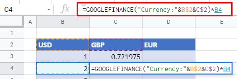

 

5. Copy the formula in this cell down to the remaining rows in our conversion table.

6. Repeat the process to look up the EUR.