Create Dynamic Drop Down From Table in Excel & Google Sheets

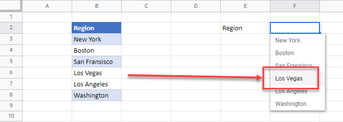
This article will demonstrate how to create a dynamic drop-down from a table in Excel & Google Sheets.

When you create a drop down list based on a range of cells using data validation, if the data in that specific range changes, then the values in the drop down list will also change.

Creating a Drop Down List

The first step in creating a drop-down list in Excel is to create the list of items in a table that will be contained within the list.

1. Type in a heading for your list (for example Region)
2. Below this heading, type in the items that will be in your drop down list.

Once you have done that, we need to format the list as a table.

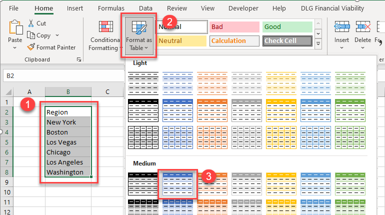
1. Select the list.
2. In the Ribbon, select Home > Styles > Format as Table.
3. Select the format type you require.

We can now create the drop down list with Data Validation.

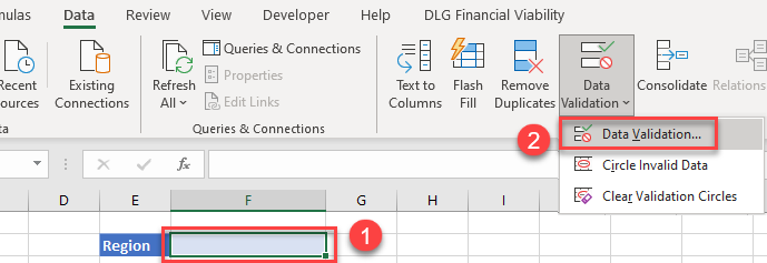
(1) select the cell where you wish the drop down list to go and then (2) in the Ribbon, select Data > Data Tools > Data Validation > Data Validation.

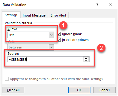
In the Settings tab, (1) select List from the Allow drop down list, and then (2) select the table data as the Source for your list.

Click on the Input Message tab to type  an input message if required

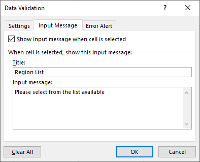
Finally, click on the Error Alert tab and type in any error message that you wish to have returned to the user.

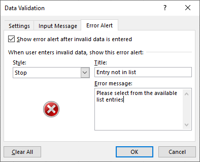
Click OK to create the drop down list.

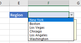
Amending the Items in the Drop Down List

To amend any item in the drop down list, you can just amend the item in your table source data.

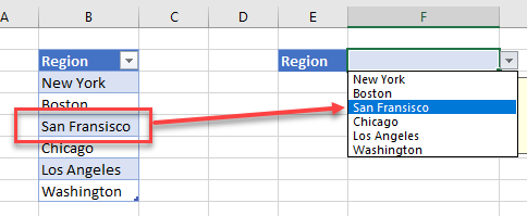
Adding or Deleting items in the Drop Down list

As your list source is an Excel table, when you add items in the table, the drop down list will automatically adjust.

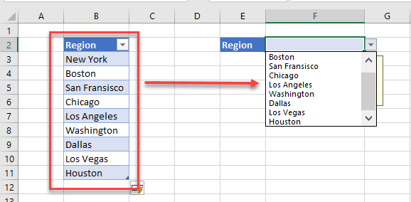
Similarly, if you delete any items from the table, they will also be removed from the drop down list.

 

Create Dynamic Drop-Down From Table in Google Sheets

We can create a drop down list in Google Sheets using a Range Name and Data Validation.

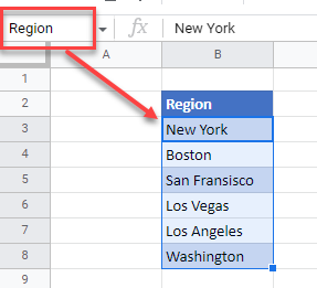
1. Type in a heading for your list (for example Region)
2. Below this heading, type in the items that will be in your drop down list.
3. Highlight all the items in the list, and then create a Range Name for the list by typing a the name for your range in the Names box.

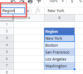
Select the cell where you wish the drop down list to be created, and then, in the Menu, select Data > Data validation.

Select “List from a range” in the criteria drop down and then type in “=” and the name of your range  eg : “=Region”

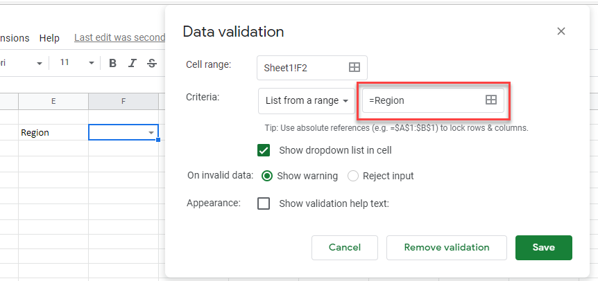
As with Excel, if you amend any of the data entries in your range name, the drop down list will automatically update.

If you delete an item from the range, then the list will also update.  However, if you wish to add an item to the list, you will need to insert a row within the range name, or, re-define your range name to include any additional rows.  This is due to the fact that Google does not support a table feature like Excel.

To insert a row into an existing range name, right-click on the row header where you wish to insert the row.

 

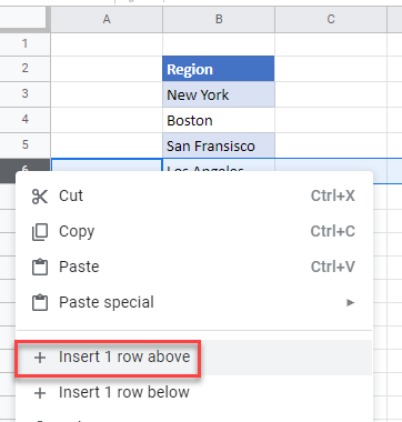
Select Insert 1 row above and then type in the additional item required.   The range name will now automatically be updated to include the additional row.

 

Click on the drop down list to see the added entry.