How to Filter Rows in Excel & Google Sheets

This tutorial will demonstrate how to filter rows in Excel and Google Sheets.

Excel enables us to store data in a table format made up of rows and columns. These tables are often in database format with the columns as the headers (database fields), and the rows as the database entries. Excel then has some fabulous database features, one of which is the ability to filter lists of data. Filtering data lists enables you to locate and report on a subset of the data.

Format Data as a Table

Once you have a list of data stored in Excel, you can choose to format the data as a table. Doing this will automatically add filters to the columns in the table.

Click in the data, and then in the Ribbon, select Home >Styles > Format as Table.

 

 

Select the type of format you wish to apply, and then, in the Format As Table dialog box, make sure the ‘My table has headers‘ is checked.

 

 

The format will be applied to the data, and a new tab called Table Design will appear in your Ribbon.

 

 

Add Filter to Excel Data

If you do not format your data as a table, you can still add filters to the data manually.

Click in your data, and then, in the Ribbon, select Home > Editing > Filter.

 

 

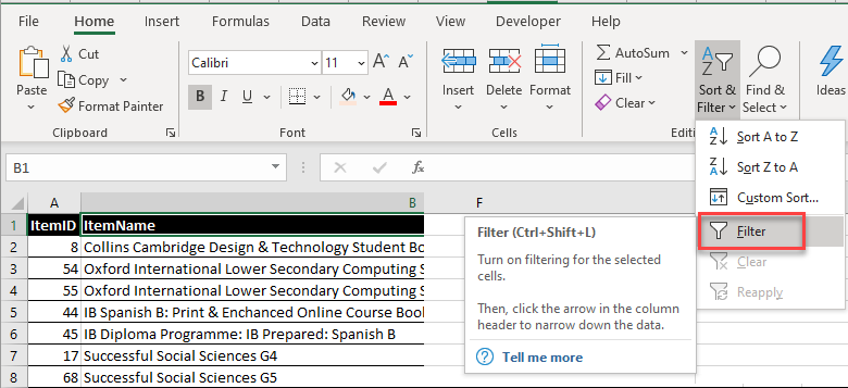
Small drop down arrows will be applied to the header row of your data.

 

 

Filter by Data in the Drop-Down List

Click on the drop down arrow to the right of the heading you wish to filter on, and then remove the check mark from Select all.

 

 

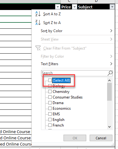
In the list of entries that is shown, click in the checkbox of the ones that you require to be shown in your filtered data.

 

 

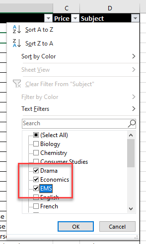
Click OK to show the data.

 

 

You will notice that the data that does not match what you have selected is hidden – the row headers turn blue as only the rows for the filtered data is shown. You will also notice that the header that you have filtered on has a small icon of a filter indicating that that column of data has the filter applied to it.

Click on the small filter to activate the drop down list. Select “Clear Filter” to remove the filter from the data.

 

 

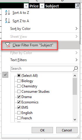
OR

select (Select All) and then click OK to remove the filter from the data.

OR

In the Ribbon, select Home > Editing > Filter > Clear.

 

 

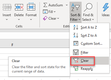
This will clear the filter from the data, but the filter headers will still remain at the top of each column of data.

Filter by Text

Click on the drop-down arrow next to the header column of the data you wish to filter, and then select Text Filters.

 

 

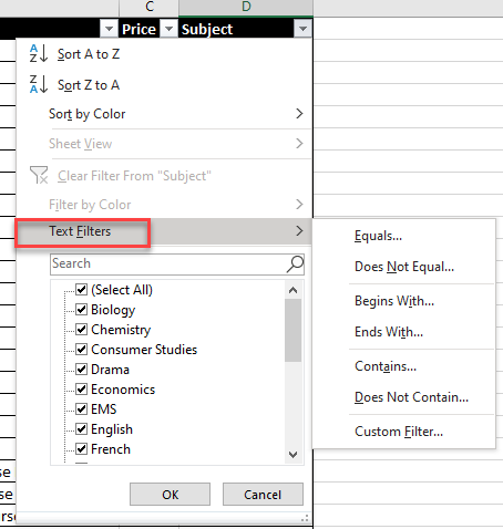
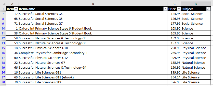
Select Contains… from the list shown and then type a word that is contained within the data e.g., “Science”

 

Click OK to filter the data.

 

 

Sort Filter

The filter drop down list has the ability to sort the filtered data.

In the filter drop down list, select Sort A to Z or Sort Z to A, depending on how you wish to sort the filtered data.

 

 

The data that is filtered will be sorted – you will notice a small arrow appearing next to the filter, indicating that the filtered data is sorted.

 

 

If we remove the filter, you will notice that the rest of the data in the list has not been sorted.

 

 

To sort the entire list of data, once the filter is cleared, you can select Sort A to Z or Sort Z to A in the filter drop down list

OR

In the Ribbon, select Home > Editing > Sort & Filter and then select Sort A to Z or Sort Z to A.

 

 

Remove Filters

To remove the filters from the data list, in the Ribbon, select Home > Editing > Sort & Filter and then click on Filter once again. This is a toggle button so will either apply filters to the list, or remove filters from the list.

 

 

Filter by Color

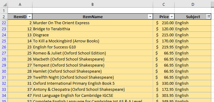
If you have formatted your data by color, Excel has the ability to filter the data based on the colors applied.

In the filter drop down, select filter by Color.

 

 

Select More Cell Colors to see all the cell colors applied to the data.

 

 

Select the color you wish to filter on, and then click OK.

 

 

Filter Rows in Google Sheets

Filtering data in Google sheets is much the same as filtering data in Excel.

In the Menu, select Data > Create a Filter.

 

 

In the drop down list, (1) click Clear to clear all the check marks from the data, and then (2) select the data items from the list.

 

 

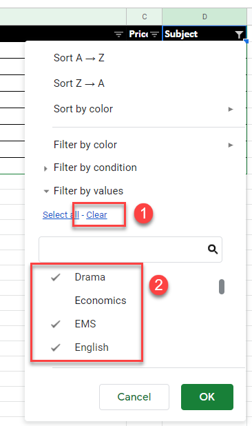
Click OK to filter the data.

 

 

To remove the filter, in the drop down list, click (1) Select All and then click (2) OK.

 

 

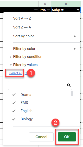
The filter will be cleared but the filter drop down will still be showing on the column headers.

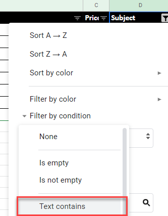
To filter the data by specific text, select Filter by condition and then in the drop down below, select Text contains. There are multiple conditions that you are able to filter on.

 

 

(1)Type in the text that you wish to filter on, and then (2) click OK.

 

 

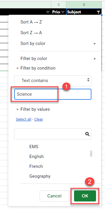
Only the rows that contain the required data will be shown.

 

 

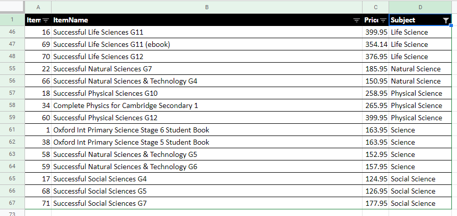
Once we have filtered our data, we can also sort the data as we can in Excel.

In the filter drop down list, select Sort A to Z or Sort Z to A, depending on how you wish to sort the filtered data.

 

 

Note that as with Excel, this will only sort the filtered data – not the entire data list.

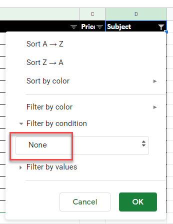
To remove the filter, select Filter by condition > None in filter the drop down list, and then click OK.

 

 

We can also filter by color in Google Sheets.

In the drop down filter list, select Filter by color > Fill color and then select one of the fill colors shown.

 

 

The data will be filtered by the color selected.

 

 

To remove the filter, select Filter by color > None in the drop down filter list.