How to Lock Columns in Excel and Google Sheets

This tutorial will demonstrate how to lock columns in Excel and Google Sheets.

Freeze Left Column

If we have a large worksheet with many columns going across the screen, we might want to make sure that we can always see the first column.

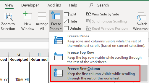
In the Ribbon, select View > Freeze Panes.

Select Freeze First Column.

As you scroll across in your worksheet, you will see that the first column remains visible regardless of how far you scroll across.

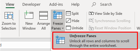
To remove the pane freeze, select Unfreeze Panes from the Freeze Panes menu.

Freeze Panes

You might want to freeze more than one column.  To do this, you can use Freeze Panes.

Position your cursor in the column you wish to freeze.

In the Ribbon, select View > Freeze Panes > Freeze Panes.

The worksheet will freeze columns A to C.  If we scroll across, these columns will remain in place.

To remove the pane freeze, select Unfreeze Panes from the Freeze Panes menu.

Freeze First Column in Google Sheets

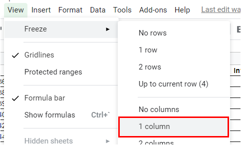
In the Menu, click View > Freeze > 1 column.

As we scroll across, the left column remains in place.

Click View > Freeze > No columns to remove the freeze.

To freeze more than one column in Google sheets, we can select either 2 columns to freeze the top 2 columns, or Up to current column(col) to freeze up to the row that you have selected.

Note that the letter in brackets after Up to current column will reflect the current column you have selected.

We can also use the Freeze Panes menus to freeze rows.