How to Merge Lists Without Duplicates in Excel & Google Sheets
In this tutorial, you will learn how to merge lists without duplicates in Excel and Google Sheets.
Merge Lists Without Duplicates
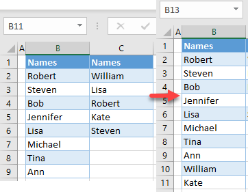
In Excel, you can merge two lists without duplicating any value by using the Remove Duplicates feature. Say you have two lists of names (in Columns B and C) like the ones in the picture below.
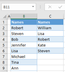
To merge these two lists in Column B and remove all duplicate values, follow these steps.
- Select and right-click a second range that will be merged (C2:C6) and click Copy (or use the keyboard shortcut CTRL + C).

- Right-click on the first empty cell after the first list (e.g., B10) and click Paste (or use the keyboard shortcut CTRL + V).
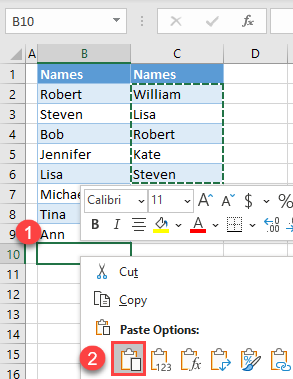
- Now you have values from both columns in Column B, but there are some duplicates.
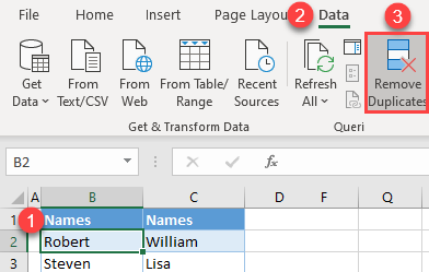
To delete the duplicates, click anywhere in the first list (B2:B15), and in the Ribbon go to Data > Remove Duplicates.
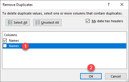
- In the pop-up window, uncheck the second column and click OK.
This will remove duplicates for the first column in your data range (Column B). The contents of the second column are irrelevant now that they’ve been copied over to Column B.
- You get the information message that three duplicate values are removed and ten unique values remain. Click OK.

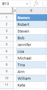
Finally, you got the merged list of values from Columns B and C in Column B, without duplicates.
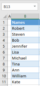
The names Lisa, Robert, and Steven are removed from the second list, as they were already present in the first list.
Note: You can also use VBA code to remove duplicates in a merged list.
Merge Lists Without Duplicates in Google Sheets
You can also merge lists without duplicates in Google Sheets.
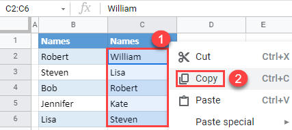
- Select and right-click a second range that will be merged (e.g., C2:C6) and click Copy (or use the keyboard shortcut CTRL + C).
- Right-click on the first empty cell after the first list (e.g., B10) and click Paste (or use the keyboard shortcut CTRL + V).
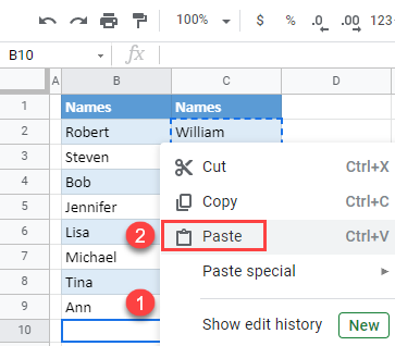
- Now you have values from both columns in Column B, but there are some duplicates.
To delete the duplicates, click anywhere in the first list (here, B2:B15), and in the Menu, go to Data > Remove duplicates.
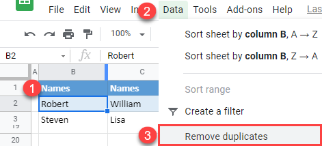
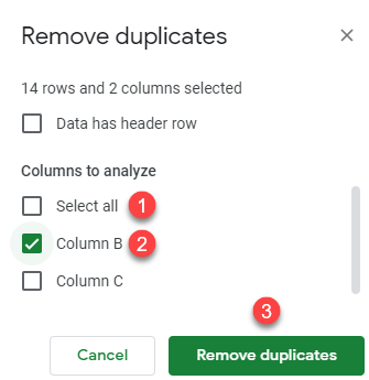
- In the Remove duplicates window, (1) uncheck Select all and (2) check Column B to compare only the values in Column B. Then (3) click Remove duplicates.
- This brings up the information pop-up below, with the number of deleted duplicates and the number of remaining unique values.

Finally, the lists are merged, with all duplicates removed, in Column B.
