Sort Multiple Rows Horizontally in Excel & Google Sheets

In this tutorial, you will learn how to sort multiple rows horizontally in Excel and Google Sheets.

Sort Single Row Horizontally

In Excel, we can use the sort option to sort rows horizontally. Let’s say that we have the following data set.

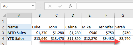
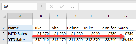
Instead of usual column data storing, in this example, we have rows-oriented data. In row 2, there are Names, while in row 3, there are month-to-date sales for every person from row 2. Also, in row 4, we have year-to-date sales. Let’s first sort data horizontally by MTD Sales from largest to smallest (row 3). To do this, follow the next steps.

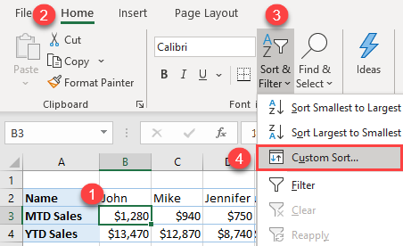
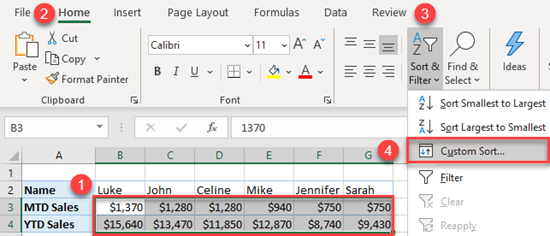
1. Click anywhere in the data range that we want to sort (A3:G3), and in the Ribbon, go to Home > Sort & Filter > Custom Sort.

 

2. In the Sort window, click Options.

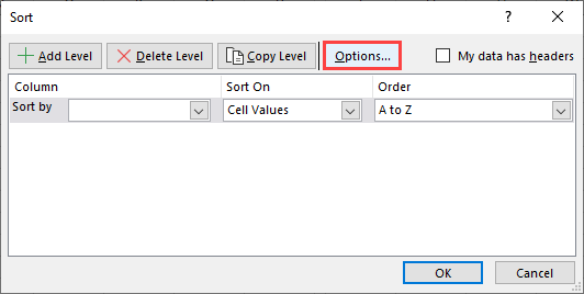
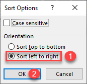
3. In the Options pop-up, select Sort left to right, and click OK. This option stands for horizontal sort, while top to bottom means vertical sort.

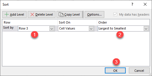
4. In the Sort window, (1) choose Row 3 for Sort by, (2) Largest to Smallest for Order, and (3) click OK.

As a result, our data set is sorted by row 3 (MTD Sales) descending.

In the sorted data, we have two times the equal amounts – for John and Celine ($1,280) and for Jennifer and Sarah ($750). In order to add additional sort criteria, we can sort multiple rows horizontally.

Sort Multiple Rows Horizontally

To be able to sort equal values for MTD Sales, we will add one more level of sorting – YTD Sales (row 4). In this case, we will first sort by MTD Sales, and then by YTD Sales, from largest to smallest. In order to achieve this, follow the next steps.

1. Select the data range that we want to sort (B3:G4), and in the Ribbon, go to Home > Sort & Filter > Custom Sort.

 

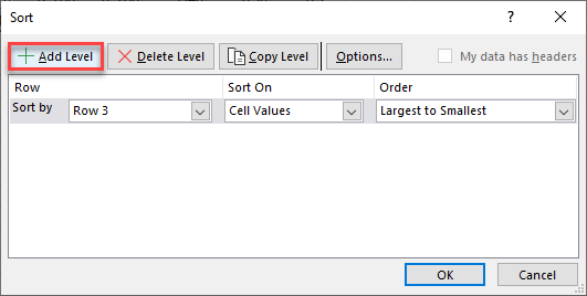
2. In the Sort window, click Add Level, to add Row 4 to the sort condition.

3. In the second level, select Row 4 for Then by, and Largest to Smallest for Order, and click OK.

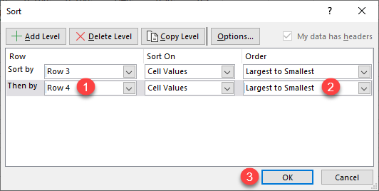
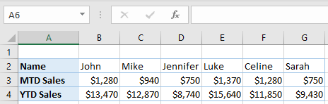
As a result, the data range is sorted first by MTD Sales, and then by YTD Sales.

 

As we can see, if there are two equal values for MTD Sales, they are sorted depending on values in YTD Sales (from largest to smallest).

Sort Single Row Horizontally in Google Sheets

Google Sheets don’t have an option like Excel to sort left to right in order to sort horizontally, but it is possible to achieve the same using the combination of the SORT and TRANSPOSE Functions. The idea is to transpose data from horizontal to vertical, then sort data, and transpose it back to horizontal. In order to achieve this, we need to enter the formula in cell A6:

=TRANSPOSE(SORT(TRANSPOSE(A2:G4),2,FALSE))

 

 

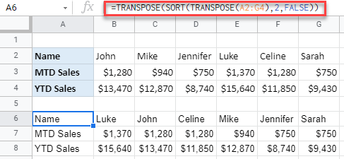
As a result, our data range is transposed below, with MTD Sales sorted descending. Let’s look deeper into the formula:

First, we transpose A2:G4, to vertical, to be able to sort it. After that, we sort that range descending (FALSE) by the second column (2 – MTD Sales). Finally, we transpose the sorted range back to horizontal.

Sort Multiple Rows Horizontally in Google Sheets

Similar to the previous example, we can sort multiple rows horizontally. The only difference is that we need to include YTD Sales in the SORT function. In this case, the formula in cell A6 is:

=TRANSPOSE(SORT(TRANSPOSE(A2:G4),2,FALSE,3, FALSE))

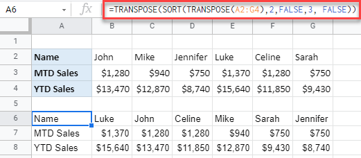
The only difference compared to the single row sort is another condition in the SORT Function. We added column 3 (YTD Sales) as a parameter, with descending sort (FALSE).