How to Use Split Screen in Excel Worksheets

This tutorial demonstrates how to use split screen in Excel.

 

 

Split Screen

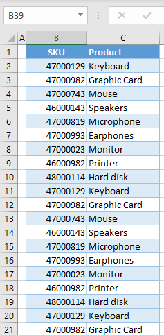
The split screen option in Excel is useful when you have a large set of data that you need to scroll through horizontally or vertically. In that case, Excel allows you to split the screen into four parts (panes) and scroll each pane independently. Every part of the screen displays the same data, but you can scroll each pane individually. This enables you to, for example, scroll in the first screen Rows 1–20, and on the second screen Rows 20–40, etc. Say you have the following data about products in Columns B and C, through Row 40.

 

 

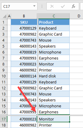
To split the screen, first decide where you want the split. Therefore, select the cell where you want to split the screen horizontally and vertically (for example B17) and in the Ribbon, go to View > Split.

 

 

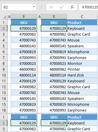
Now, the screen is split into four panes that can be scrolled independently.

 

 

When the screen split is active, columns left from the split point and above it, will always be fixed. In this case, the fixed part is Column B in the left pane and Rows 1–16 in the upper pane. Basically, with the screen split, you have the same data displayed in four panes of the window. If you select for example cell B2 and scroll the bottom screen up, you will see that B2 is selected on all four screen panes.

 

 

This Excel feature is useful when you have large sets of data to compare. Then, you can split the screen and have one part of the data fixed, while scrolling the other part. To turn off the split screen option, go back to View > Split.