INDEX MATCH MATCH – Excel & Google Sheets

This tutorial will demonstrate how to perform a 2-Dimensional lookup with the INDEX and MATCH Functions in Excel and Google Sheets.

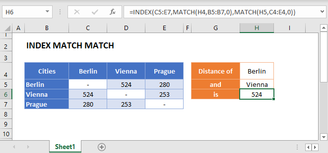
Match Two Axis –  Row & Column (2D Lookup)

The INDEX Function returns a value from a given Row and Column reference. We can supply both the row and column references with MATCH functions to perform a 2d-lookup:

=INDEX(C3:E5,MATCH(H2,B3:B5,0),MATCH(J2,C2:E2,0))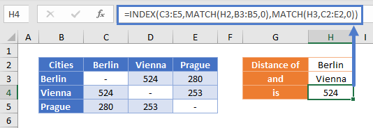

 

Let’s go into the details.

MATCH Function

To find the row, use the MATCH Function with your first value.

=MATCH("Berlin",B3:B5,0)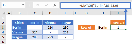

This finds the row containing “Berlin” and returns its position within the given range. “Berlin” is the 1st city in Column B, so the MATCH Function returns 1.

Then we repeat for the column we are interested in.

=MATCH("Vienna",C2:E2,0)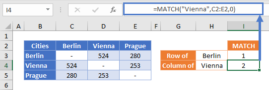

“Vienna” is the 2nd city, so the MATCH Function returns 2.

INDEX Function

Now that we have the positions for the row and column, we use them as arguments in the INDEX Function to return the value of the cell where they intersect (here, the distance from Berlin to Vienna).

=INDEX(C3:E5,I3,I4)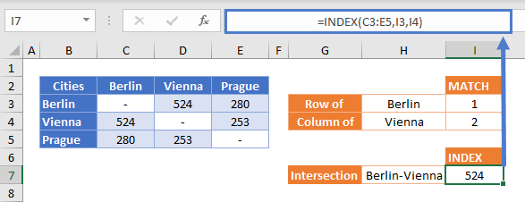

Replacing the column and row numbers with the MATCH Functions that found them gives us our original formula:

=INDEX(C3:E5,MATCH(H2,B3:B5,0),MATCH(J2,C2:E2,0))

INDEX MATCH MATCH in Google Sheets

These formulas work exactly the same in Google Sheets as in Excel.