Excel Reference Cell in Another Sheet or Workbook – Excel and Google sheets

Download Example Workbook

Download the example workbook

This tutorial will demonstrate how to reference a cell in another sheet in Excel and Google Sheets

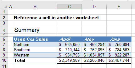
Reference to another Sheet – Create a Formula

In a workbook with multiple worksheets, we can create a formula that will reference a cell in a different worksheet from the one you are working in.

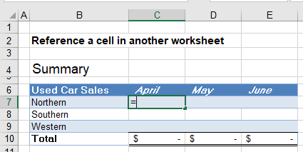
Select the cell where the formula should go ex: C7

Press the equal sign, and then click on the sheet you wish to reference.

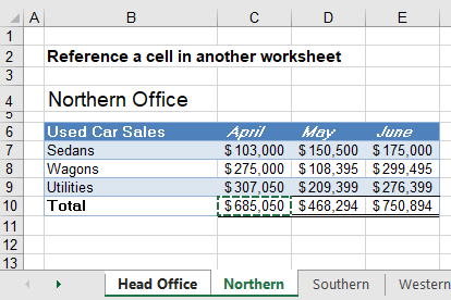
reference cell in another sheet workbook 02

Click on the cell that holds the value you require.

reference cell in another sheet workbook 03

Press Enter or click on the tick in the formula bar.

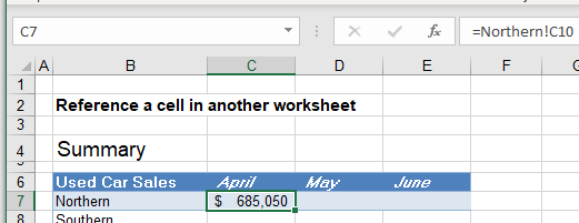
reference cell in another sheet workbook 04

Your formula will now appear with the correct amount in cell C7.

The sheet name will always have an exclamation mark at the end. This is followed by the cell address.

Sheet_name!Cell_address

For example:

=Northern!C10

If your sheet name contains any spaces, then the reference to the sheet will appear in single quotes.

For example:

='Northern Office'!C10

Should the value change in the source sheet, then the value of this cell will also change.

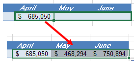
You can now drag that formula across to cells D7 and E7 to reference the values in the corresponding cells in the source worksheet.

reference cell in another sheet workbook 05

Reference to Another Sheet – the INDIRECT Function

Instead of typing in the name of the sheet, you can use the INDIRECT Function to get the name of the sheet from a cell that contains the sheets name.

reference cell in another sheet workbook 06

When you reference another sheet in Excel, you usually type the sheet’s name, and then an exclamation mark followed by the cell reference. Since sheet names often contain spaces, we often enclose the name of the sheet in single quotes.

In the formula above therefore, we have used the INDIRECT Function to refer to the name of the sheet in cell B7 ex: “Northern”.

The entire formula above would therefore be

=INDIRECT("'" & Northern & "!C10")

where we have replaced the sheet name “Northern” with cell B7.

We can then copy that formula down to C8 and C9 – and the sheet name “Northern” will be replaced with “Southern” and “Western” as the formula is copied down.

Reference to another Sheet – an Array Formula

To reference to another sheet using an Array formula, select the cells in the Target worksheet first.

For example:

Select C8:E8

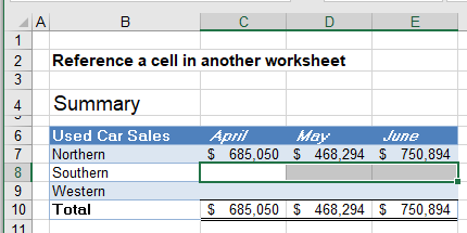
reference cell in another sheet workbook 07

Press the equal sign, and then click on the worksheet that contains the Source data.

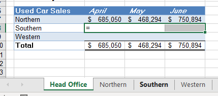
reference cell in another sheet workbook 08

Highlight the relevant source data cells.

reference cell in another sheet workbook 09

Press Enter to enter the formula into the Target worksheet.

reference cell in another sheet workbook 10

You will notice that the cells contain a range (C10:E10) but that each relevant column will only show the value from the corresponding column in the source workbook.

Reference to a Range Name

The array formula is useful when you are referencing to a range name that contains a range of cells and not just a single cell.

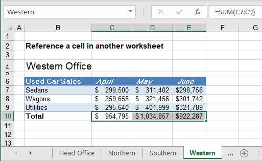
reference cell in another sheet workbook 11

In the above example, the total values of the Western office in row 10 is called Western.

Click in the Head Office sheet, highlight the cells required and press the equal sign on the keyboard.

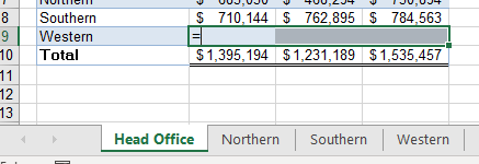
reference cell in another sheet workbook 12

Type the range name that you have created ex: Western.

reference cell in another sheet workbook 13

Press Enter.

reference cell in another sheet workbook 14

An array formula will be created.

Reference to another Workbook

You can also link workbooks together by means of referencing to a cell in another workbook.

reference cell in another sheet workbook 15

Have both workbooks open in Excel. You can use the view menu to see them both on the screen if you wish.

Click in the cell you wish to put the source data in ex: C12

Press the equal key on the keyboard and click on the Source cell in the different Workbook.

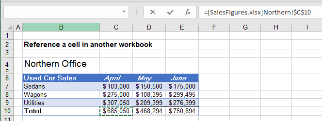
reference cell in another sheet workbook 16

Press Enter.

The formula that is entered into the original sheet will have a reference to the external file, as well as a reference to the sheet name in the external file.

The name of the workbook will be put into square brackets, while the sheet name will always have an exclamation mark at the end. This is followed by the cell address.

[Workbook_name]Sheet_name!Cell_address

For example:

=[SalesFigures.xlsx]Northern!$C$10

You will notice that the cell reference has been made an absolute. This means that you CANNOT drag it across to columns D and E unless you remove the absolute.

Click in the cell, and then click in the formula bar and click on the cell address of the formula bar.

Press F4 until the absolute is removed.

Alternatively, you can delete the $ signs from around the absolute.

Drag the formula across to columns D and E.

reference cell in another sheet workbook 18

Reference to another Sheet in Google Docs

Linking worksheets with formulas works the same way in Google Docs as it does in Excel.

Click in the cell you wish to put the formula into, and then click on the Source cell where your value is stored.

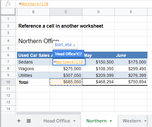
reference cell in another sheet workbook 19

Press Enter.

Your formula will now appear with the correct amount in cell C7.

The sheet name will always have an exclamation mark at the end. This is followed by the cell address.

Sheet_name!Cell_address

For example:

=Northern!C10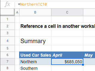

reference cell in another sheet workbook 20

Drag the formula across to populate columns D and E, and then repeat the process for all the sheets.

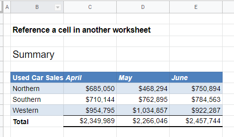
reference cell in another sheet workbook 21

Reference to another Sheet using an Array Formula in Excel

The array formula will also work in the same way.

Highlight the range you wish to put the target information in and press the equal sign on the keyboard.

reference cell in another sheet workbook 22

Click on the Source sheet and highlight the cells you require.

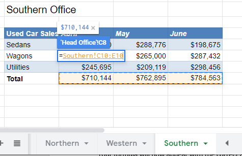
reference cell in another sheet workbook 23

Press Shift+Enter.

reference cell in another sheet workbook 24

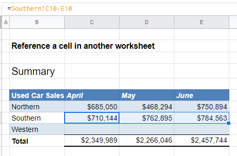
The formula will appear as a range but that each relevant column will only show the value from the corresponding column in the source workbook.

reference cell in another sheet workbook 25

Reference to another Workbook in Google Docs

If you want to link Google Sheets files together, you need to use a function called IMPORTRANGE

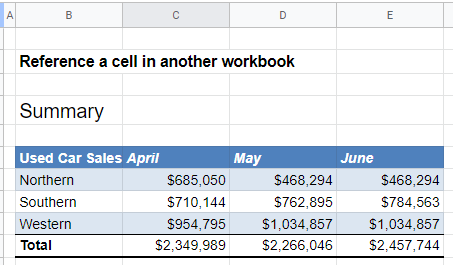
reference cell in another sheet workbook 26

Open the Source Google sheet file in order to copy the URL address of the file.

For example

reference cell in another sheet workbook 27

Return to the sheet where you wish to input the formula and click in the relevant cell.

Press the equal sign on the keyboard and type in the function name ex: IMPORTRANGE, followed by a bracket and inverted commas.

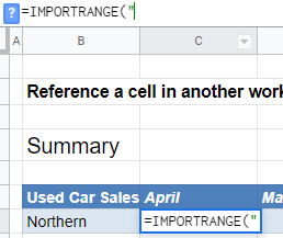
reference cell in another sheet workbook 28

Paste the URL copied from the source Google sheet into the formula.

Close the inverted commas

For example:

=IMPORTRANGE("https://docs.google.com/spreadsheets/d/1kJ9ECcuwO65ayFXCobxuUSwx9MnPSDXypiyPWoHc59E/edit#gid=1711678147"

Add another comma and then also in inverted commas, type in the cell reference required

For example

“Northern!C10”

Your complete formula will look like the example below

=IMPORTRANGE("https://docs.google.com/spreadsheets/d/1kJ9ECcuwO65ayFXCobxuUSwx9MnPSDXypiyPWoHc59E/edit#gid=1711678147", "Northern!C10")

When you link Google sheets for the first time, this message could appear.

reference cell in another sheet workbook 29

Click Allow access.

Repeat the process for any other cells that need to be linked eg D10 and E10.

TIP: Drag the formula across to the required cells and change the cells address in the formula bar!

reference cell in another sheet workbook 30