Sum Values if Dates are Equal– Excel & Google Sheets

This tutorial will demonstrate how to use the SUMIFS Function to sum data with specific dates in Excel and Google Sheets.

Sum Values if Dates are Equal

The SUMIFS Function sums data that meet certain criteria. Its syntax is:

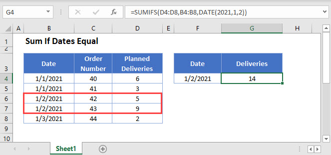
This example will sum the number of Planned Deliveries on a specific Date by using the SUMIFS and DATE Functions.

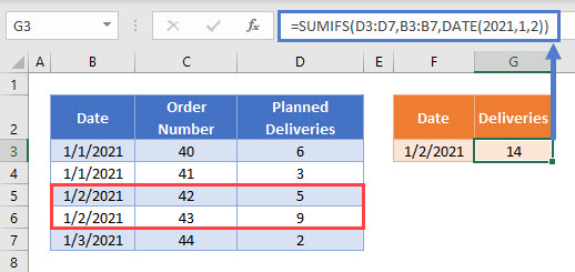
=SUMIFS(D3:D7,B3:B7,DATE(2021,1,2))

In this example, we want to sum Deliveries planned for 1/2/2021. To enter this Date as a criteria in our formula, we use the DATE Function:

DATE(2021,1,2)

In this case, the DATE Function expression above is all we need to test whether the date is equal to 1/2/2021. However, a logical test in the SUMIFS Function generally requires an operator in double quotes (“”), so the sum criteria could also be written as:

"="&DATE(2021,1,2)

Sum Values if Dates are Equal – Cell References

Usually, it is bad practice to hard-code date values into formulas. Instead, it is more flexible to use a separate cell to define the date to be used as a sum criteria.

=SUMIFS(D3:D7,B3:B7,F3)

This allows the user to change the Date used in the formula in a quicker and more visual way by editing the cell F3.

Note that other logical operators can also be used in SUMIFS, such as:

• Greater than (“>”&F3)
• Greater than or equal to (“>=”&F3)
• Less than (“<“&F3)
• Less than or equal to (“<=”&F3)
• Not equal to (“<>”&F3)

Locking Cell References

To make our formulas easier to read, we’ve shown the formulas without locked cell references:

=SUMIFS(D3:D7,B3:B7,F3)

But these formulas will not work properly when copy and pasted elsewhere in your file. Instead, you should use locked cell references like this:

=SUMIFS($D$3:$D$7,$B$3:$B$7,F3)

Read our article on Locking Cell References to learn more.

Sum Values if Dates are Equal in Google Sheets

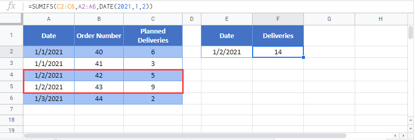
These formulas work exactly the same in Google Sheets as in Excel.