TEXTJOIN IF- Excel & Google Sheets

This tutorial will demonstrate how to concatenate cell values based on criteria using the TEXTJOIN Function in Excel and Google Sheets.

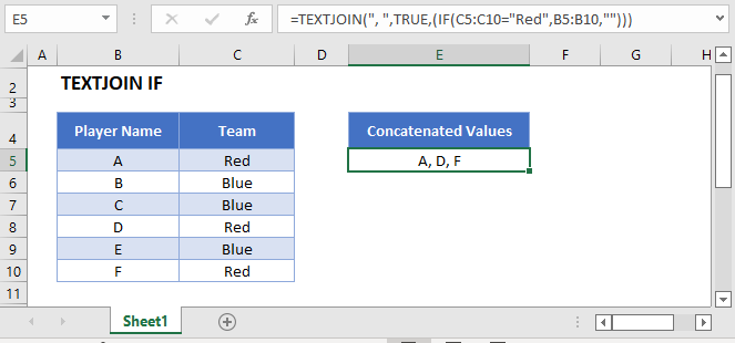
The TEXTJOIN Function

Users of Excel 2019+ have access to the TEXTJOIN Function, which merges multiple strings of text together, separating each string with a specified delimineter.

Note: Google Sheets users can use the TEXTJOIN Function, but have a slightly different way of entering array formulas. See the later section on this topic.

This example will use the TEXTJOIN and IF Functions in an array formula to create a comma separated text string of Player Names which relate to a Team value of Red

=TEXTJOIN(", ",TRUE,IF(C3:C8="Red",B3:B8,""))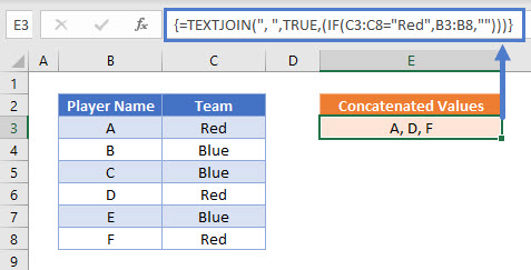

Users of Excel 2019 will need to enter this formula as an array function by pressing CTRL + SHIFT + ENTER. Users of later versions of Excel do not need to follow this step.

To explain what this formula is doing, lets break it down into steps:

This is our final formula:

=TEXTJOIN(", ",TRUE,IF(C3:C8="Red",B3:B8,""))

First, the cell range values are added to the formula:

=TEXTJOIN(", ",TRUE,IF({"Red"; "Blue"; "Blue"; "Red"; "Blue"; "Red"}="Red",{"A"; "B"; "C"; "D"; "E"; "F"},""))

Next the list of Team names is compared to the value Red:

=TEXTJOIN(", ",TRUE,IF({TRUE; FALSE; FALSE; TRUE; FALSE; TRUE},{"A"; "B"; "C"; "D"; "E"; "F"},""))

The IF Function replaces TRUE values with the Player Name, and FALSE values with “”

=TEXTJOIN(", ",TRUE,{"A"; ""; ""; "D"; ""; "F"})

The TEXTJOIN Function then combines all of the array values into one text string. We have instructed the function to ignore blank values and to add the text “, ” between each value. This produces the final result:

="A, D, F"

 

TextJoin If – pre-Excel 2019

As the TEXTJOIN Function is not available before the Excel 2019 version, we need to solve this problem in a different way. The CONCATENATE Function is available but does not take ranges of cells as inputs or allow array operations and so we are required to use a helper column with an IF Function instead.

This next example shows how to use a helper column to create a comma separated text string of Player Names which relate to a Team value of Red:

=IF(C3="Red",B3&", ","")&D4

The first step in this example is to use an IF Function to replicate the condition of Team = Red. If the condition is met, the Player Name value is written and followed by the chosen delimiter “, “:

=IF(C3="Red",B3&", ","")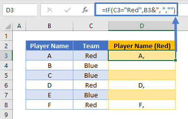

Next, we can create a column that builds up a list of these values into one cell by also referencing the cell below it:

=D3&E4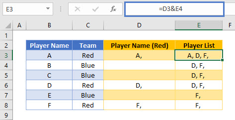

This formula uses the & character to join two values together. Note that the CONCATENATE Function could be used to create exactly the same result, but the & method is often preferred as it is shorter and makes it clearer what action the formula is performing.

These two helper columns can then be combined into one formula:

=IF(C3="Red",B3&", ","")&D4

A summary cell can then reference the first value in the Player List helper column:

=D3

If the final “,” value is not required, an additional nested IF Function should be added to the formula:

=IF(C3="Red",IF(D4="",B3,B3&", "),"")&D4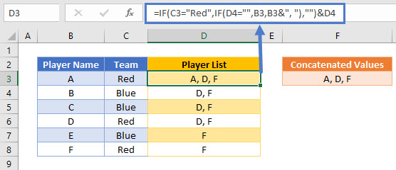

The additional part of the formula is the IF Function below:

IF(D4="",B3,B3&", ")

 

This part of the formula checks the value of the cell below it. If it is empty, then this cell must be the last Player Name in the list and the name is written without a delimiter. If the cell below contains a value, then this cell is not the last Player Name in the list and so the “, ” delimiter is added.

TextJoin If in Google Sheets

These formulas work the same in Google Sheets as in Excel, except that the ARRAYFORMULA Function is required to be used in Google Sheets for it to evaluate the results correctly. This can be automatically added by pressing the keys CTRL + SHIFT + ENTER while editing the formula (or by manually add:

=ARRAYFORMULA(TEXTJOIN(", ",TRUE,(IF(C3:C8="Red",B3:B8,""))))