This tutorial demonstrates how to use the TEXTJOIN Function in Excel and Google Sheets to combines text from multiple strings.

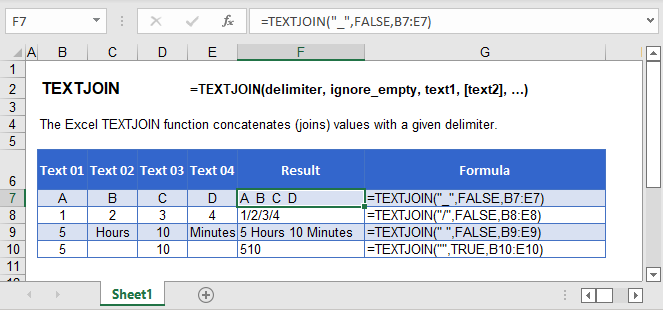
TEXTJOIN Function Overview

The TEXTJOIN Function combines text from multiple strings. You can specify your choice of delimiter (comma, semi-colon, space, line break, etc.) and whether to ignore blank values. It is available in Excel 2016 and above.

It’s syntax is:

=TEXTJOIN (delimiter, ignore_empty, text1, [text2], ...)

delimiter – Separator between each text.

ignore_empty – Whether to ignore empty cells or not.

text1 – First text value or range.

text2 – [optional] Second text value or range.

This example will combine First and Last Names, separated by a delimiter (the character that splits the word) and a choice to include blanks (next example will be more obvious).

=TEXTJOIN(" ",false,B3:C3)

TEXTJOIN to Include Blanks

If the second argument is set to FALSE, blank values are concatenate like other text.

=TEXTJOIN(";",FALSE,B3:E3)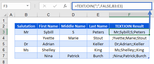

This might be what you want, as it makes it easy to split the text again. However, in some cases you won’t want this…

TEXTJOIN to Ignore Blanks

It would not make sense to include blanks if the scenario is to combine the salutation with the names like this below:

=TEXTJOIN(" ",FALSE,B3:E3)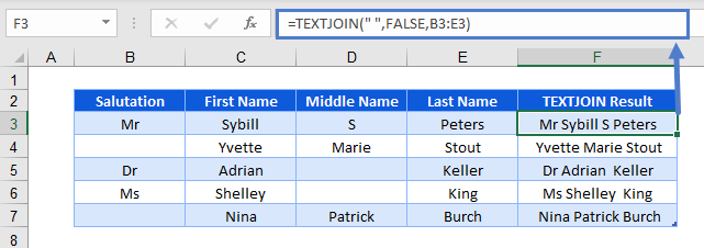

You can see the obvious ones in F5 and F6 where there is an extra space between the first and last names.

In this scenario, it would be better to ignore blank cells if they are not filled with a TRUE as the second argument.

=TEXTJOIN(" ",TRUE,B3:E3)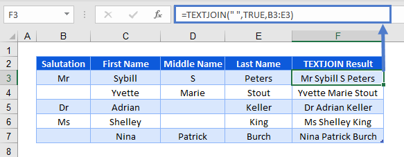

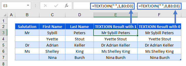
TEXTJOIN with 1 and 0

If you’ve used VLOOKUP, you might know Excel recognizes TRUE as 1 and FALSE as 0. They can be used interchangeably in most cases.

TEXTJOIN with Condition

You might want to combine the text, only if they meet a condition. In this scenario, you might want to join the Full Names with commas as the delimiter, only if it’s “Yes” in Worked Overtime (column C).

{=TEXTJOIN(", ",TRUE,IF(C3:C7="Yes",B3:B7,""))}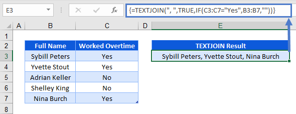

This is an array formula.

If you’re using a version of Excel prior to 2019, you must press CTRL + SHIFT + ENTER instead of ENTER after typing the formula. You should see curly brackets surrounding it when done right (DO NOT manually type the curly brackets).

If you’re using Excel 2019 or Office 365, you can enter the formula normally.

TEXTJOIN with Different Delimiters

You can use array constants (the curly brackets) to input multiple delimiters like this:

=TEXTJOIN({"-","."},1,B3:D3)

It will know to use a dash (-) as the first delimiter and period (.) as the second one.

TEXTJOIN with Number/Date

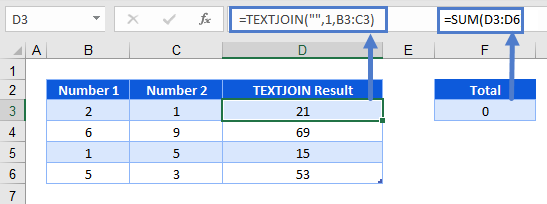
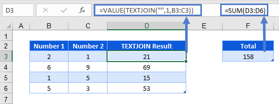
When using TEXTJOIN, the result is always text. Notice in this example, we join together 2 numbers. The resulting number will be stored as text and numerical functions will not work

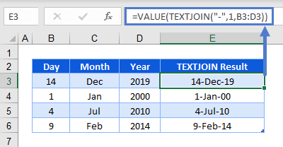
The same thing happens for dates.

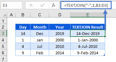
To overcome the issues above, you can use VALUE to convert from text to values.

Other Examples of TEXTJOIN

Reverse a String of Text

You can reverse a text string by combining MID Function with TEXTJOIN as follow.

=TEXTJOIN("",1,MID(A2,{10,9,8,7,6,5,4,3,2,1},1))

Which would give us the following results:

TEXTJOIN Function in Google Sheets

The TEXTJOIN function works almost the same in Google Sheets.