VLOOKUP Returns 0? Return Blank Instead – Excel & Google Sheets
Download the example workbook
This tutorial will demonstrate how to return blank if VLOOKUP’s output is blank. If your version of Excel supports XLOOKUP, we recommend using XLOOKUP instead.

In Excel, when referring to another cell with a formula, blank values are calculated as zero.

This can be a problem for some VLOOKUP scenarios where we need to distinguish blanks from zeroes:
=VLOOKUP("2021-D",B3:C7,2,FALSE)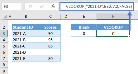
VLOOKUP with IF and ISNA
We can use the combination of VLOOKUP with IF and ISNA to solve this problem:
=IF(ISBLANK(VLOOKUP(E3,B3:C7,2,FALSE)),"",VLOOKUP(E3,B3:C7,2,FALSE))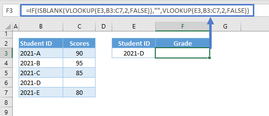
Let’s breakdown and analyze the formula:
To return blank if the VLOOKUP output is blank, we need two things:
- A method to check if the output of the VLOOKUP is blank
- And a function that can replace zero with an empty string (“”), which is the closest to blank that we can return.
ISBLANK Function
We can use ISBLANK to check if the result of VLOOKUP is blank.
=ISBLANK(VLOOKUP(E3,B3:C7,2,FALSE))
Notes:
- The ISBLANK Function returns TRUE if a value is blank. Empty string (“”) and 0 are not equivalent to a blank. A cell containing a formula is not blank, and that’s why we can’t use F3 as input for the ISBLANK.
- Formulas can return blanks, but they are converted to zero at the final stage of the calculation.
- Therefore, we can nest formulas in ISBLANK to check if their results are blanks rather than assigning the formulas to cells before applying ISBLANK to the cells.
IF Function
We can then use the IF Function to test whether the combination of ISBLANK and VLOOKUP is TRUE or FALSE. We can set any process (e.g., output an empty string) if the condition is TRUE and another one (e.g., the result of the VLOOKUP if not blank) if the result is FALSE.
=IF(G3,"",F3)
Combining all of these concepts results to our original formula:
=IF(ISBLANK(VLOOKUP(E3,B3:C7,2,FALSE)),"",VLOOKUP(E3,B3:C7,2,FALSE))
VLOOKUP with IF and Empty String (“”)
We can use the empty string as a criterion to check if the value of the VLOOKUP is blank instead of using the ISBLANK Function:
=IF(VLOOKUP(E3,B3:C7,2,FALSE)="","",VLOOKUP(E3,B3:C7,2,FALSE))
Note: Blank can be equivalent to zero or empty string depending on the calculation, but empty strings and 0s are not blanks.
VLOOKUP with IF and LEN
Another alternative to ISBLANK is the by using the LEN Function:
=IF(LEN(VLOOKUP(E3,B3:C7,2,FALSE))=0,"",VLOOKUP(E3,B3:C7,2,FALSE))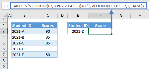
Let’s dive deeper into this alternative solution:
Check If Blank using LEN
As stated earlier, formulas do return blank results but are converted at the end of the calculations.
Therefore, we can use the LEN Function to count the number of characters of the VLOOKUP’s output:
=LEN(VLOOKUP(E3,B3:C7,2,FALSE))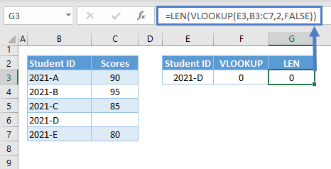
If the number of characters is 0, this means that the value is blank. We can then use the IF Function to check if the LEN Function is equal to 0, and return an empty string if this is true:
=IF(G3=0,"",F3)
Combining all of these concepts results to our original formula:
=IF(LEN(VLOOKUP(E3,B3:C7,2,FALSE))=0,"",VLOOKUP(E3,B3:C7,2,FALSE))
VLOOKUP Return Blank in Google Sheets
All aforementioned formulas work the same way in Google Sheets, and in fact, we don’t need to implement them in Google Sheets to display a blank-like result because Google Sheets can return blanks.
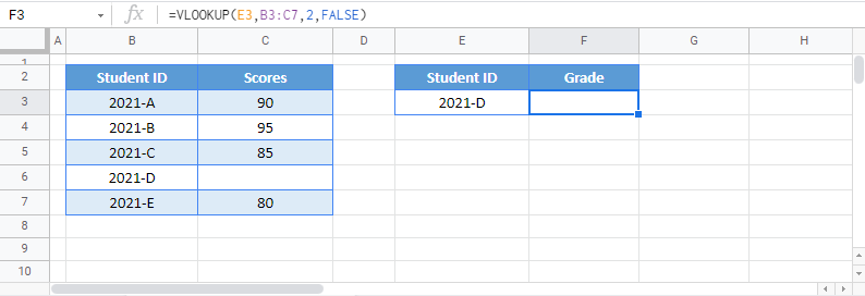
Note: This is very helpful in scenarios where we need to distinguish blanks from empty strings.
Take note that the formulas above are only applicable if the output is blank, which is different from a “no match” result. If VLOOKUP doesn’t find a match, it will return the #N/A Error instead, and in this case, we need to handle the #N/A Error; please see the article: “VLOOKUP – Fix #NA Error”