XLOOKUP Duplicate Values

This tutorial will demonstrate how to XLOOKUP duplicate values in Excel. If your version of Excel does not support XLOOKUP, read how to use the VLOOKUP duplicate values instead.

Lookup Duplicate Values

In Excel 365, looking up duplicate values is easier thanks to the FILTER Function. We will demonstrate the FILTER Function first and then demonstrate how to lookup duplicate values with XLOOKUP.

With the FILTER Function, just enter the array (e.g., Scores) that we want to return and the criteria range (e.g., Student ID) with the criteria (e.g., 2021-A).

=FILTER(C3:C7,B3:B7=E2)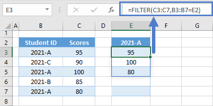

 

We can also nest the FILTER Function inside the INDEX Function and input a row_num (e.g., F3) to return an nth match that we want instead of returning all the matches.

=INDEX(FILTER(C3:C7,B3:B7=E3),F3)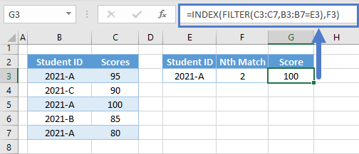

 

The above scenarios showcase the FILTER Function as the more convenient solution to those types of problems in Excel 365. However, lookup scenarios that require a list of lookup values are often better solved through XLOOKUP formulas because we can convert them to dynamic array formulas, which makes them more flexible than the FILTER Function.

Let’s look first at the non-dynamic array solution to break down how it works before using the dynamic array XLOOKUP.

 

XLOOKUP – Duplicate Lookup Values

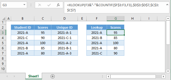
Let’s say you want to lookup a list of duplicate values using the XLOOKUP Function. Below, on the right, we have our lookup values. On the left we have the lookup table. We want to lookup each duplicate value and output in separate rows.

 

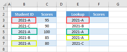
We can use the non-dynamic array formula solution below:

=XLOOKUP(F3&"-"&COUNTIF($F$3:F3,F3),$D$3:$D$7,$C$3:$C$7)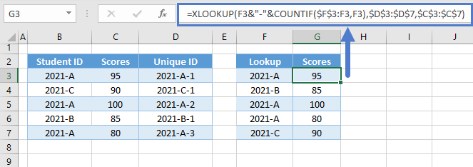

 

Let’s walk through the formula:

Unique ID – COUNTIF

First, we join the original ID (e.g., Student ID) with the COUNTIF Function to create a list of unique IDs that will distinguish the 1^st entry of an item from its duplicates.

=B3&"-"&COUNTIF($B$3:B3,B3)

 

Locking one part of the range reference inside the COUNTIF Function enables us to count the occurrence of a value as the range expands.

=COUNTIF($B$3:B3,B3)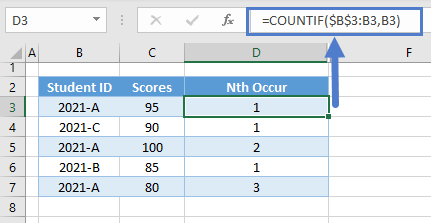

Now, we use the & Operator to stitch the COUNTIF Function to the original ID. We also added a separator (e.g., “-“).

=B3&"-"&D3

 

Combining everything together results to our Unique ID Formula:

=B3&"-"&COUNTIF($B$3:B3,B3)

 

Duplicate Lookup Values – Nth Match

Just like with the original ID, we also need to create a list of unique IDs for the lookup values. Applying the same method:

=G3&"-"&COUNTIF($G$3:G3,G3)

 

XLOOKUP Function

Now, we input the new lookup array and list of lookup values to the XLOOKUP Function:

=XLOOKUP(H3,$E$3:$E$7,$C$3:$C$7)

 

XLOOKUP – Duplicate Lookup Values (Dynamic Array)

Instead of adding new columns and copying or dragging formulas, we can convert the previous XLOOKUP Formulas into one dynamic array formula that can generate the same output.

Here’s how it looks:

=XLOOKUP(E3:E7&"-"&COUNTIF(OFFSET(E3,0,0,SEQUENCE(ROWS(E3:E7))),E3:E7),
B3:B7&"-"&COUNTIF(OFFSET(B3,0,0,SEQUENCE(ROWS(B3:B7))),B3:B7),
C3:C7)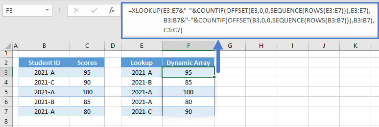

 

Let’s walk through the formula above:

Just like with the previous method, we first need to create a list of unique IDs using the COUNTIF Function. The challenge would be how to create an array formula that will generate an array of range references (e.g., B3, B3:B4, B3:B5 and so on).

 

OFFSET-SEQUENCE-ROWS Formula

We can use the combination of the OFFSET, SEQUENCE and ROWS functions to return an array of range references.

Let’s start with the list of lookup array (e.g., B3:B7):

=OFFSET(B3,0,0,SEQUENCE(ROWS(B3:B7)))

Note: The formula above won’t work on its own. Excel can’t return an array of ranges or arrays, but it can evaluate it as we will see later.

 

ROWS Function

First, we need to determine the total number of rows using the ROWS Function.

=ROWS(B3:B7)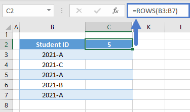

SEQUENCE Function

Next, we input the result of the ROWS Function in the SEQUENCE Function to generate a list of counting numbers, which also represents the number of cells per range in the array of ranges.

=SEQUENCE(C2)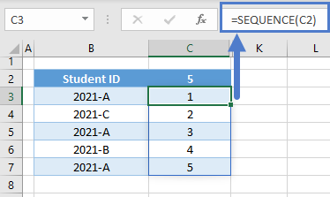

Array OFFSET Formula

Next, we input the results of the SEQUENCE Function to the height (4^th argument) of the OFFSET Function to build the ranges.

=OFFSET(B3,0,0,C3:C7)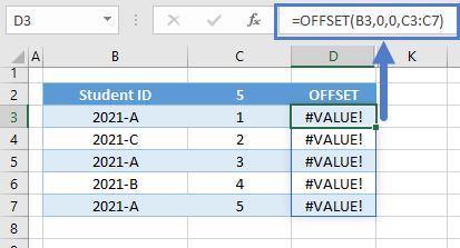

As mentioned earlier, this won’t work, but this is how the array of ranges is supposed to look like:

 

We start with B3 and expand it for each height (e.g., C3:C7).

 

Note: OFFSET if a volatile function, which means that it recalculates whenever there’s a spreadsheet change even if it’s not related to the inputs of the OFFSET itself.

 

Array COUNTIF Function

Now that we have an array of ranges, we input it to the COUNTIF Function and return an array of nth occurrences.

=COUNTIF(OFFSET(B3,0,0,C3:C7),B3:B7)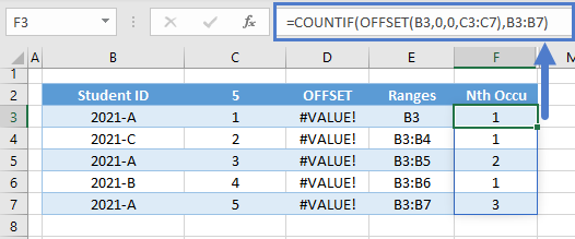

Array Unique ID

Finally, we concatenate the array output of the COUNTIF Function to the lookup array (e.g., B3:B7) to generate the array of unique IDs.

=B3:B7&"-"&F3:F7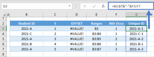

Combining all the functions results to our array Unique ID Formula:

=B3:B7&"-"&COUNTIF(OFFSET(B3,0,0,SEQUENCE(ROWS(B3:B7))),B3:B7)

 

We also do the same for the lookup values:

=I3:I7&"-"&COUNTIF(OFFSET(I3:I7,0,0,SEQUENCE(ROWS(I3:I7))),I3:I7)

Combining everything together results to our original array formula:

=XLOOKUP(E3:E7&"-"&COUNTIF(OFFSET(E3,0,0,SEQUENCE(ROWS(E3:E7))),E3:E7),
B3:B7&"-"&COUNTIF(OFFSET(B3,0,0,SEQUENCE(ROWS(B3:B7))),B3:B7),
C3:C7)