RANDBETWEEN Function Examples in Excel, VBA, & Google Sheets

This tutorial demonstrates how to use the RANDBETWEEN Function in Excel and Google Sheets to calculate a random number between two numbers.

How to use the RANDBETWEEN Function in Excel:

The RANDBETWEEN Function generates a random number (whole numbers only) between two numbers.

This formula will generate a random number between 1 and 100.

=RANDBETWEEN(B3,C3)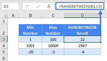

Note: RANDARRAY is a new function in Excel 2019 onwards that replaces the RANDBETWEEN Function. But if you don’t have the latest version or need to send the file out for people who don’t have it yet, you still can use the RANDBETWEEN function for backwards compatibility.

Besides generating random numbers you specify, RANDARRAY allows you to choose how many rows and columns to place the random numbers, and you can even choose if you want whole numbers or decimals.

If your Excel version is Excel 2003 or before, you will need to use RAND instead.

=RAND()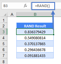

Generate Decimals Within a Range

As mentioned, RANDARRAY and RAND can generate random decimal values automatically. With RANDBETWEEN, you need to divide by a multiple of 10 to create a decimal value:

=RANDBETWEEN($B$3*10,$B$6*10)/10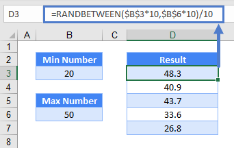

You need to first decide how many decimal places you want. In the above eg, it’s one decimal place. And you need to divide a whole number by 10 to get one decimal place. Hence, the formula is basically

=RANDBETWEEN(Minimum Number x 10, Maximum Number x 10) / 10.

Generate Random Dates or/and Time

Dates and time are stored in Excel as serial numbers. So it’s easy to generate a random date:

=RANDBETWEEN($B$3,$B$6)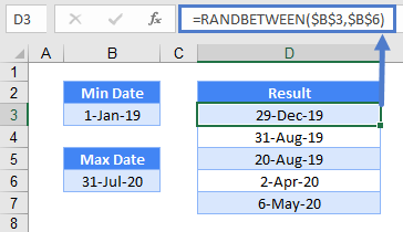

In Excel, times are stored as decimal values, where the decimal value represents a fraction of a day. There are 24 hours a day, so multiply the minimum and maximum numbers by 24 and divide that random number by 24 to get a random hour.

=RANDBETWEEN($B$3*24,$B$6*24)/24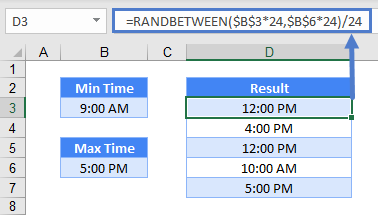

If you want random minutes as well, use 1440 (24 hours x 60 minutes) instead of 24.

=RANDBETWEEN($B$3*1440,$B$6*1440)/1440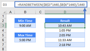

To have them both together, simply add them together:

=RANDBETWEEN($B$3,$B$6)+RANDBETWEEN($C$3*1440,$C$6*1440)/1440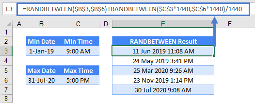

Retrieve a Random Field

The RANDBETWEEN Function can be used to retrieve a random field. Let’s look at an example of returning a random employee from a range (ex. B3:B7). Use the INDEX Function to return the employee corresponding to the random number.

=INDEX(B3:B7,RANDBETWEEN(1,5))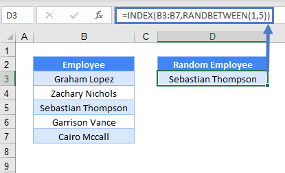

Retrieve a Random Field Without Duplicates

To return random values, without duplicates, you can use this array formula.

{=INDEX($B$3:$B$7,LARGE(IF(ISNA(MATCH($B$3:$B$7,D$2:D2,0)),ROW($B$3:$B$7),0),
RANDBETWEEN(1,5-ROWS(D$3:D3)+1))-ROW($B$3)+1)}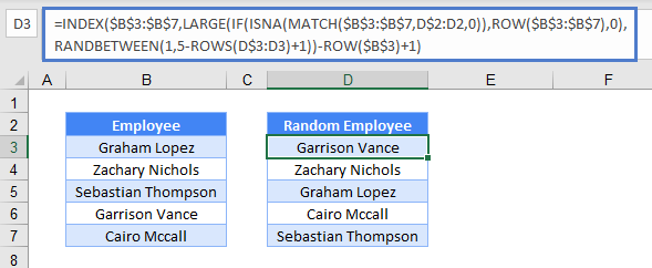

Note: Don’t type the brackets ({). Press CTRL + SHIFT + ENTER to enter the formula.

In the above eg, RANDBETWEEN first randomizes between 1 and (5 – ROWS(D$3:D3) + 1). As you copy this formula down the randomize range shrinks from (1 to 5) to (1 to 1). By doing this, we avoid duplicates.

The IF + ISNA + MATCH + ROW functions are used to only return a row number that’s not already in use.

RANDBETWEEN Function in Google Sheets

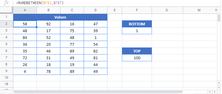
The RANDBETWEEN function works the same in Google Sheets.

 

RANDBETWEEN Examples in VBA

You can also use the RANDBETWEEN function in VBA. Type: Application.Worksheetfunction.Randbetween(bottom,top)
For the function arguments (bottom, etc.), you can either enter them directly into the function, or define variables to use instead.

Executing the following VBA statements

Range("C2") = Application.WorksheetFunction.RandBetween(Range("A2"), Range("B2"))
Range("C3") = Application.WorksheetFunction.RandBetween(Range("A3"), Range("B3"))
Range("C4") = Application.WorksheetFunction.RandBetween(Range("A4"), Range("B4"))

will produce the following results

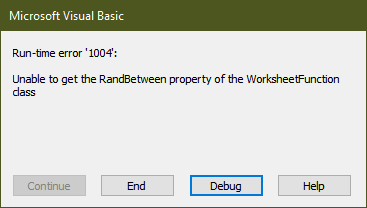
The third statement will raise an error, as RANDBETWEEN will not accept negative numbers as parameters: