Add Percentage Style to a Number in Excel & Google Sheets
This tutorial demonstrates how to style a number with a percentage sign in Excel and Google Sheets.
Add Percentage Style to a Number
In Excel, you can format a list of numbers as percentages. Say you have the following list of numbers in Column B.
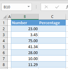
To format numbers from Column B as percentages, you need to use a separate column (C).
- Column C should have the values from Column B divided by 100, so in cell C2, enter the formula:
=B2/100
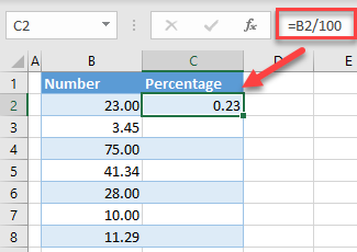
- Position the cursor in the bottom right corner of cell C2, and when it turns to a black cross, drag it to the end of the range (C8).
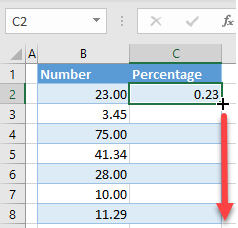
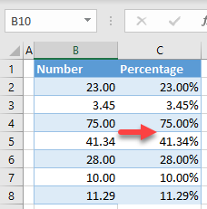
- Now you have all numbers from Column B divided by 100 in Column C. Select the range with the divided numbers (C2:C8) and in the Ribbon, go to Home > Number > Percentage (%).
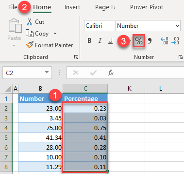
As a result, the values in Column C are formatted as percentages
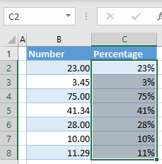
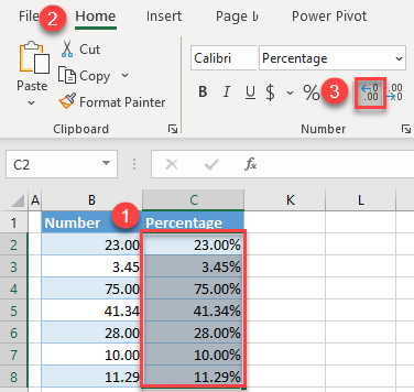
As you can see above, the default for percentages is zero decimal places. If you want to add decimal numbers to percentages, (1) select the range with percentage values, and in the Ribbon, (2) go to the Home tab. Here, (3) click on the Increase Decimal icon in the Number group. Every click will add one decimal position, so click twice to add 2 decimal numbers.
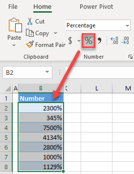
The reason you have to use an extra column (C) is that Excel, when formatting numbers as percentages, doesn’t adjust the whole number to a percentage value. So, if you have 34.5 and convert it to a percentage, it’ll be 345%.
See also: Formatting Numbers in Excel VBA.
Add Percentage Style to a Number in Google Sheets
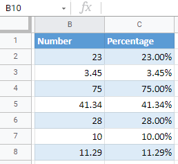
In Google Sheets, you can also add the percentage style to a number. As in Excel, you need a helper column with whole numbers divided by 100 (see Step 1 in the section above).
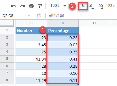
- Select the cells with decimal numbers (C2:C8), and in the Menu, click the Percentage symbol.
- To add decimals, select the range with percentages (C2:C8), and in the Menu, click the Increase decimal places icon.
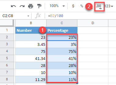
All values from Column B now have percentage style in Column C.
