How to Alternate Row Color in Excel & Google Sheets
This tutorial demonstrates how to alternate row color in Excel and Google Sheets.
Alternate Row Color
Table Formatting
To format each row in a table to have alternate row colors, you can use the Format as Table feature in Excel.
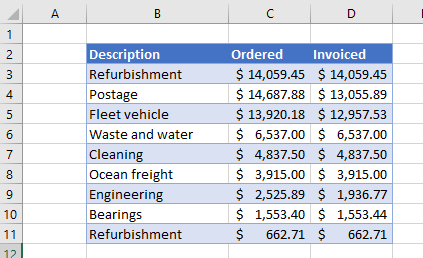
- Select the cells you wish to apply the alternate row colors or click in the middle of the range of cells you wish to apply the alternate row colors to.

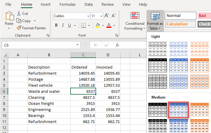
- Then, in the Ribbon, select Home > Styles > Format as Table and then select the type of formatting required.
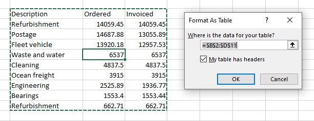
- If applicable, make sure the My table has headers box is checked and click OK.
The data is formatted as a table, with alternative row colors.
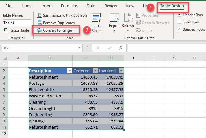
- Notice there is (1) a new Table tab on the Ribbon.
Click (2) Convert to Range to convert the table back into a simple range of cells.
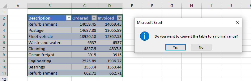
- Click OK to convert the table to a normal range.
OR
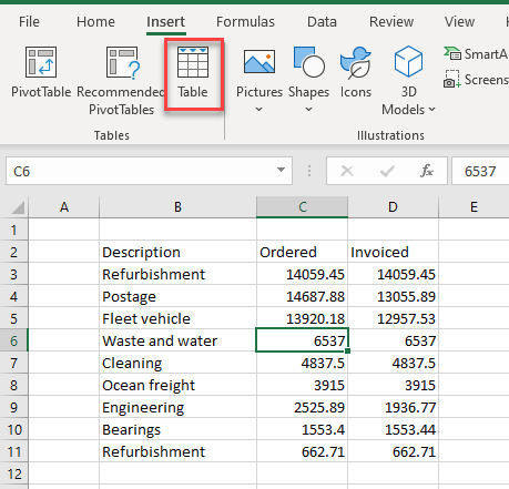
Another way to format data as a table (Steps 1–3 above) is through the Ribbon’s Insert tab.
- In the Ribbon, select Insert > Table.
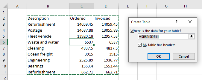
- Once again, check the My table has Headers check box if relevant.
Conditional Formatting
You can also create alternative colors for each row using Conditional Formatting.
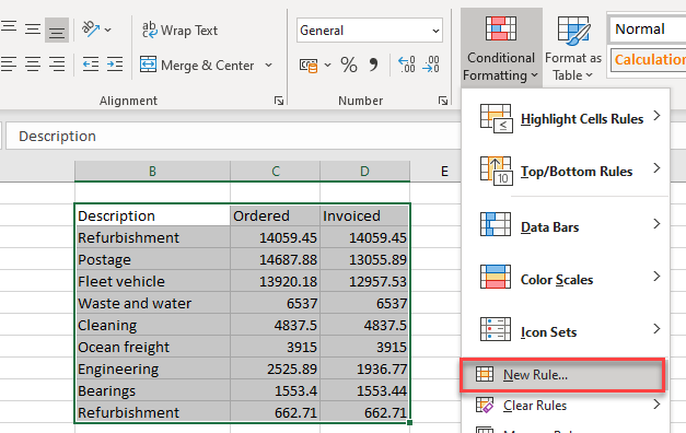
- Select the cells you wish to apply the alternate row colors to, and then, in the Ribbon, select Home > Styles > Conditional Formatting, and then select New Rule.
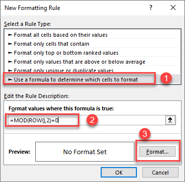
- In the New Formatting Rule dialog box, select (1) Use a formula to determine which cells for format.
Then, (2) type in this formula:
=MOD(ROW(),2)=0Next, click (3) on Format.
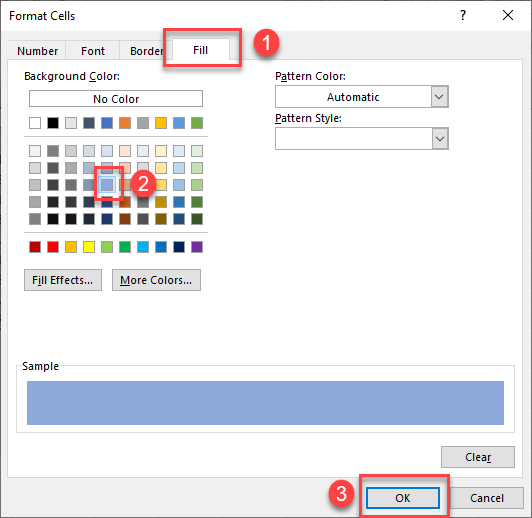
- In the Format Cells dialog box, select (1) the Fill tab and (2) select the Background Color. Finally (3) click on OK and then click OK again to return to Excel.
As you can see below, the data has alternating colors.

Alternate Row Color in Google Sheets
Alternate Colors
- Select the cells you wish to apply the alternate row colors or click in the middle of the range of cells you wish to apply the alternate row colors to.
- In the Menu, select Format, Alternate Colors.

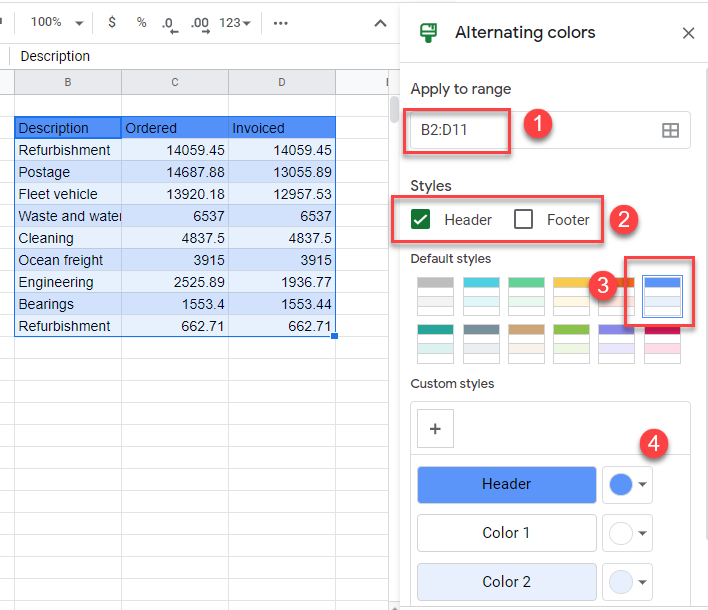
- The entire table will automatically be selected in the (1) Apply to range box. In the Styles (2) a Header is automatically selected – you can remove the tick if you do not wish to have a header row. You can (3) select the style you require, or (4) you can create a Custom style and select your own colors for the Header and alternate rows.
- Click Done when complete to apply the format to the Google Sheet.
Conditional Formatting
You can also apply alternate colors in Google Sheets using Conditional Formatting.
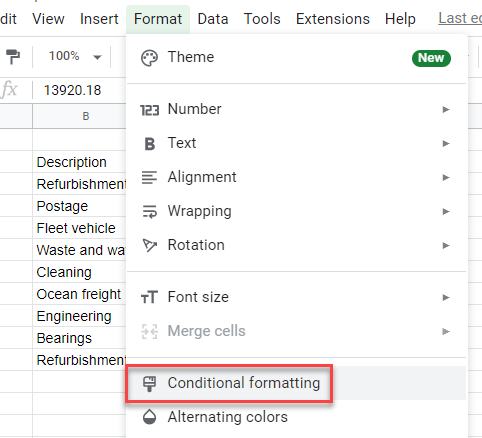
- Select the cells you wish to format, and then, in the Menu, select Format > Conditional Formatting.
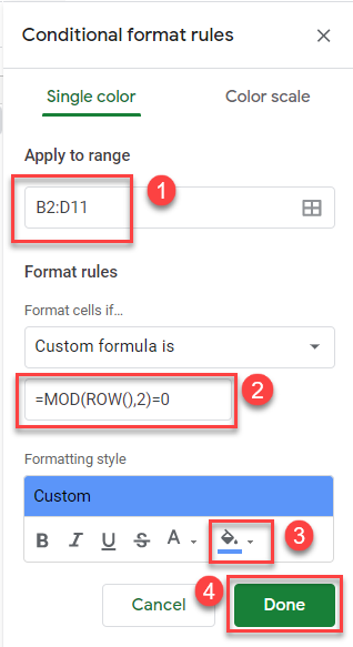
Make sure the (1) range is correctly selected and then select Custom formula is in the Format cells dropdown list.
- You can use the same formula from the Excel example above.
=MOD(ROW(),2)=0- Select the background color of the cells.
- Then click Done.
Again, you get alternating colors.
