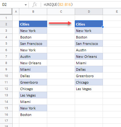
Working With Distinct / Unique Values in Excel & Google Sheets

This article will demonstrate how to work with distinct values in Excel & Google Sheets.

 

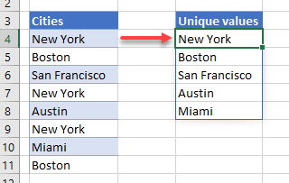
If you have a sheet of data in Excel that contains repetative data, you might need to find a way to extract unique values out of this data.  There are a few different functions that we can use in order to find these unique values.

The UNIQUE Function

To extract unique values out of a list of values in Excel that contains duplicates.  We can use the new UNIQUE Function to do this.  This function is only available in Excel 365.

Consider the following list of values:

The list in column B contains repetative names of cities.   To extract the unique values from this list, click in D3 and type the following formula:

=UNIQUE(B3:B16)

 

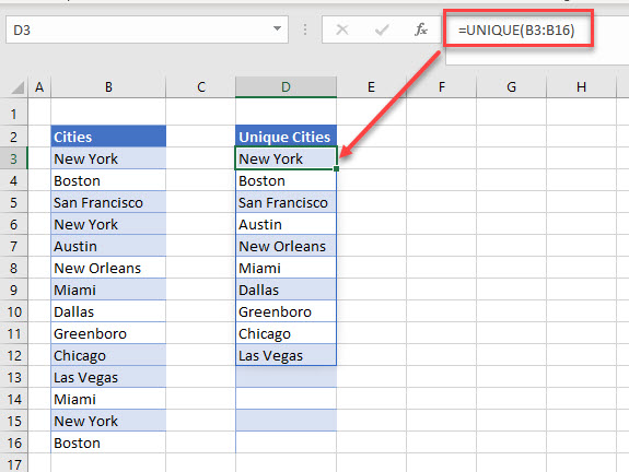
When you press Enter to enter your formula into the worksheet, it will automatically populate the rows below with the unique values from Column B.   Any cities that are repeated are therefore only shown once.

You will notice that if you move your pointer to cell D4, the formula in D4 is greyed out – you are not able to amend it.

 

 

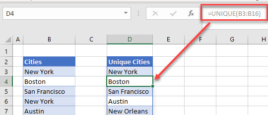
This is because the list is automatically filled in by the formula contained in cell D3 – you can only amend or delete the formula if you have D3 selected.

Finding Unique Values in Multiple Columns (Unique Rows)

We can also use the unique function to list unique rows of data containing multiple columns.

Consider the following worksheet:

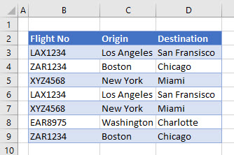
We have a list of flights with their origin and destination.    As we can see in the data, there are rows that are identical and are repeated.

To extract the unique values, type this formula in F3:

=UNIQUE(B3:D9)

 

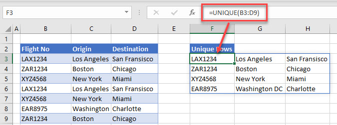
As with the single column formula, the range of cells will automatically be filled with the unique rows as duplicate rows are only shown once.

Unique Values with the INDEX, MATCH, COUNTIF AND ISERROR Functions

If you are using a version of Excel prior to Excel 365, or using Excel 2019, you will not have the UNIQUE function available.

To extract unique values from a list will then require a bit more work.

The general formula we will use is this:

=IFERROR(INDEX(B$3:B$10,MATCH(0,COUNTIF(D$2:D2, B$3:B$10),0)),"")

As you can see in the above formula, we are combining the IFERROR, INDEX, MATCH and COUNTIF functions.

Four built in Excel functions are required to achieve the same result that the new UNIQUE function achieves in Excel 365.

NOTE: The formula has to all be written as one, it will not work when broken into sections so we need to explain it as it is shown in the example above.

The COUNTIF Function

The COUNTIF Function is used to Count values that appear according to certain criteria.

Consider this section of the formula

COUNTIF(D$2:D2, B$3:B$10)

The Range to be Counted is D$2:D2 (which at the moment does not have a match from the range in column B so would return a 0.

As the formula is copied down, the range to count would alter according to the mixed address (D$2:D3) would change to D$2:D4, D$2:D5 etc – until the final row where it would be D$2:D10.

The MATCH Function

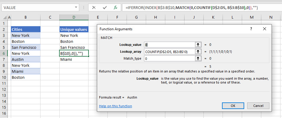
The MATCH Function is then used to return the row that matches the value returned by the COUNTIF function.

For this section of the formula in Row 3 the result is 1 as the formula is looking up the value of 0 in the array.  As it finds a match in the row, it returns a value of 1 for that row.

MATCH(0,COUNTIF(D$2:D2, B$3:B$10),0)

As we copy the formula down, the COUNTIF Function will add 1 to the result it produces.  The MATCH Function is looking for zeros, not ones – so it will return the position of the next available zero in the list.  In row 6 for example, it will return 5 as the matching row.

 

The INDEX Function

The INDEX function then returns the data contained in the row returned by the MATCH function.

INDEX(B$3:B$10,MATCH(0,COUNTIF(D$2:D2, B$3:B$10),0))

In row 3, the value “New York” is returned.

As the formula is copied down, if we were to look in row 10, then a different value would be returned.

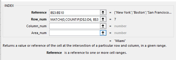
However, if we were to look in row 22, an error would be returned.

The ISERROR Function

To prevent this error from showing up in the sheet, the ISERROR function is used as the final function in the formula.

If an error is returned, the ISERROR function will return a blank text string to the cell instead of the #N/A that the index section of the formula would return.

=IFERROR(INDEX(B$3:B$10,MATCH(0,COUNTIF(D$2:D2, B$3:B$10),0)),"")

Find Unique Records with a Pivot Table

As with other methods in working with unique records, select the range of cells that you wish to obtain your unique records from.

Then, in the Ribbon, select  Insert > Tables > Pivot Table.

 

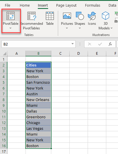
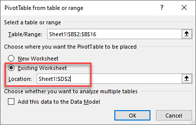
Select a location in the Existing Worksheet to place your pivot table.

 

In the Pivot Table fields list, drag the field down to the Row area of the Pivot table.

 

Only unique values will now be shown in the Pivot table.

 

Find Unique Values with Conditional Formatting and Filter by Color

We can use Conditional Formatting to find unique values in our data, and then we can use the Filter by color function to show just these values.

As with other methods in working with unique records, select the range of cells that you wish to obtain your unique records from.

Then, in the Ribbon, select Home > Styles > Conditional Formatting > New Rule.

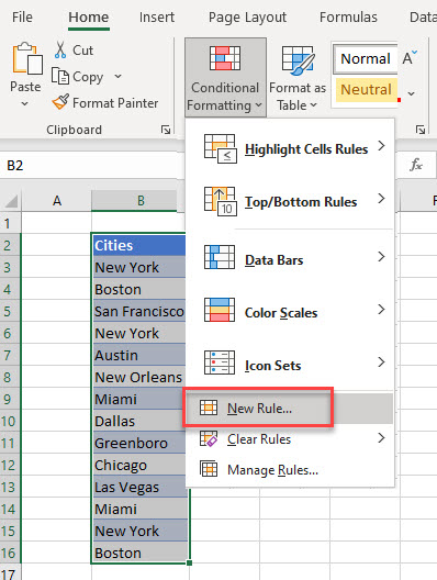
(1) Select “Format only unique or duplicate values” and then, in the Format all drop down, (2) select unique.  Finally, (3) set the format you require.

Click OK to apply the rule.

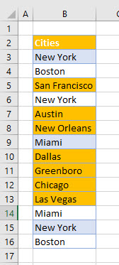
Now, in the Ribbon, select Home > Editing > Sort & Filter > Filter and then select Filter by Color in the filter drop down list.

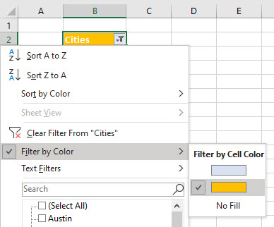
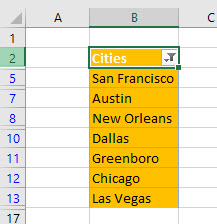
The unique values will now be filtered and shown in your worksheet.

 

Find Unique Values Using Advanced Filter

You can also use an advanced filter to find unique values.

Select a cell in the list you wish to filter, and then, in the Ribbon, select Data > Sort & Filter > Advanced.

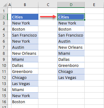
In the Advanced Filter dialog box, make sure (1) Copy to another location is selected.   Then (2), enter or select the location to copy the records to and finally (3), make sure Unique records only is selected.

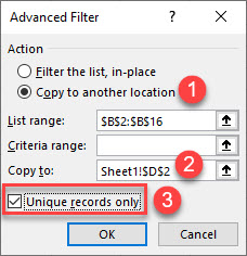
Click OK to filter your records.

 

Find Unique Values with VBA

Finally, we can also find unique values using the RemoveDuplicates function in VBA.    

Sub RemoveDups()
  Range("B2:B16").RemoveDuplicates Columns:=1, Header:=xlYes
End Sub

Working With Distinct / Unique Values in Google Sheets

Google sheets does not have VBA or Pivot Tables but every other method used above to obtain unique values in Excel can also be used in Google sheets.