How to Hide Formulas in Excel & Google Sheets

This tutorial shows how to hide formulas in Excel.

 

 

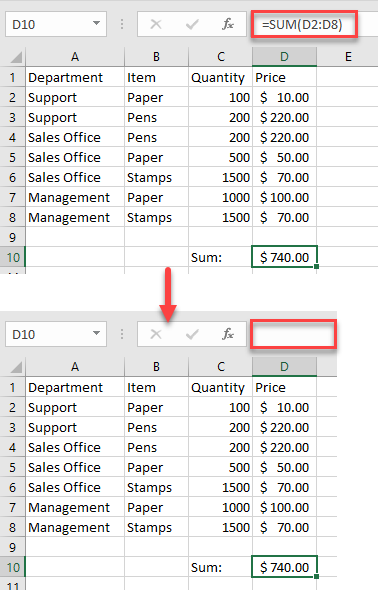
Hide Formulas in Excel

In Excel, if a cell contains a formula, that formula is displayed in the formula bar when the cell is selected. But if you don’t want to display formulas for proprietary, security, or confidentiality reasons, you can easily hide them.

 

 

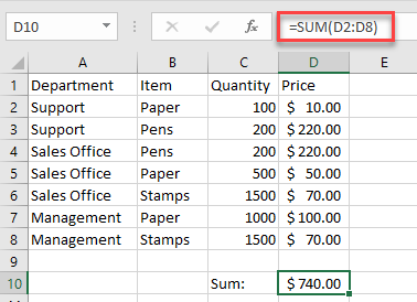
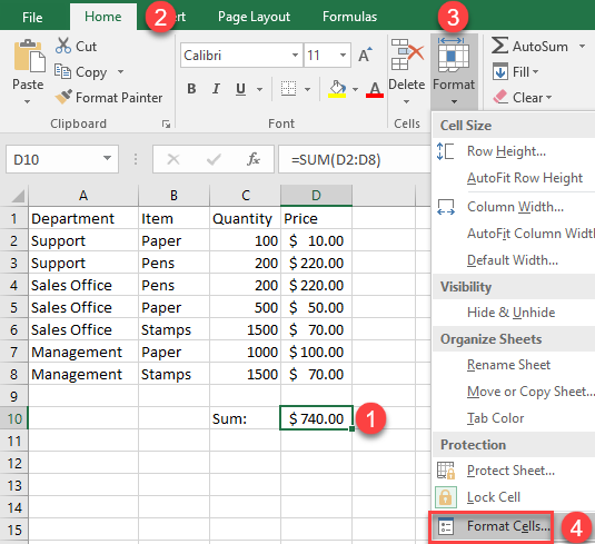
1. Select the cell with the formula you want to hide, then in the Ribbon go to Home > Format > Format Cells.

 

 

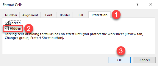
2. In the Format Cells window, go to Protection, check the box next to Hidden, and click OK.

 

 

3. To make the formula-hiding feature work, you need to protect your workbook. In the Ribbon, go to Review and click on Protect Sheet.

 

 

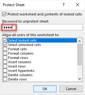
4. In the Protect Sheet window, type in a password and press OK.

 

 

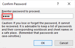
5. In the Confirm Password window, reenter the password and click OK.

 

 

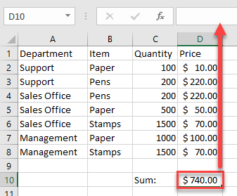
As a result, the formula is locked and hidden. When you click on the cell, you won’t be able to see the formula in the formula bar.

 

 

Hide the Formula Bar

Another way to hide the formula is to hide the whole formula bar. In the Ribbon, go to View and uncheck the box next to the Formula Bar.

 

 

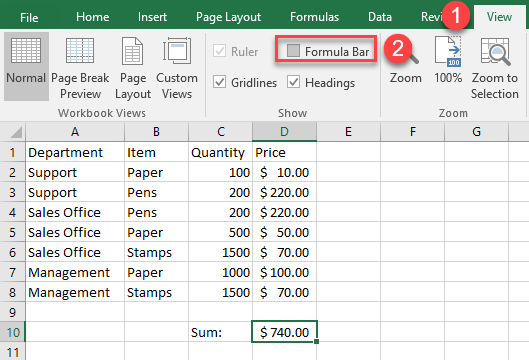
Keep in mind this won’t actually hide the formula for protection reasons. Anyone can enable the Formula Bar later and see the formula.

Hide Formula Bar in Google Sheets

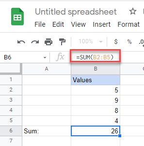
Say you have a formula in cell B6 and want to hide it. In Google Sheets, you can’t hide this formula the same way you can in Excel; but what you can do is hide the whole formula bar.

 

 

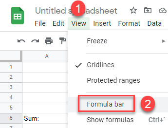
In the Menu, go to View > Formula bar to disable this option.

 

 

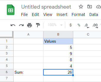
Now, the formula bar is hidden, and you won’t be able to see the formula.

 

 

Alternatively, if you want to protect the formula from further edits you can lock the cell as a protected range.