How to Lock Cells in Excel & Google Sheets

This tutorial demonstrates how to lock cells in Excel and Google Sheets.

 

 

Lock All Cells

In Excel, you can lock all cells for editing. To do this, password protect a sheet.

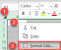
1. By default, all cells in Excel have the property Locked turned on, and you can check this (1) by selecting all cells (click the arrow in the upper left corner of the gridlines), (2) right-click anywhere in the selected area, and (3) choose Format Cells…

 

 

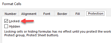
2. In the Format Cells window, go to the Protection tab, and here you can see that Locked is checked. This means that, when you protect your sheet, all cells are locked for editing.

 

 

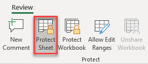
3. Now you can protect the sheet. In the Ribbon, go to Review > Protect Sheet.

 

 

4. In the Protect Sheet window, enter a password and press OK. As you can see, after you protect the worksheet, users will only be able to select cells.

 

 

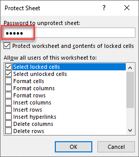
5. In the pop-up window, confirm the password and press OK.

 

 

Now, if you try to edit any cell in the sheet, you’ll get the message that the sheet is protected and can’t be edited.

 

 

To be able to edit cells again, unprotect the sheet.

Lock Specific Cells

To lock only a specific range of cells (for example, B1:B3), follow these steps:

1. Select all cells (by clicking on the arrow in the upper left corner of the gridlines), (2) right-click anywhere in the selected area, and (3) choose Format Cells…

 

 

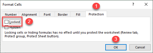
2. In the Format Cells window, (1) go to the Protection tab, (2) uncheck Locked, and (3) click OK.

 

 

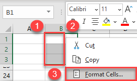
3. Now, (1) select cells you want to lock (here, B1:B3), (2) right-click anywhere in the selected area, and (3) choose Format Cells…

 

 

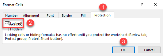
4. In the Format Cells window, (1) go to the Protection tab, (2) check Locked, and (3) click OK.

 

 

As a result, you can edit all cells except B1:B3 which are locked.

 

 

In the picture above, you can see that cell B4 is edited, but when you try to edit any cell in the range B1:B3, you get the error message.

Note that you also have the option to lock only formatting.

Lock Cells in Google Sheets

You can also lock cells for editing in Google Sheets, using protected ranges.

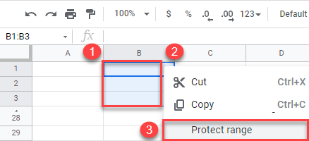
1. Select all cells (by clicking on the arrow in the upper left corner of the gridlines), (2) right-click anywhere in the selected area, and (3) choose Protect range.

 

 

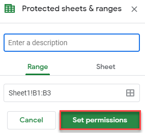
2. In the window on the right side, choose Set permissions.

 

 

3. Here, you can choose to only show a warning, or to specify who can edit the range (you or another specific user). Then click Done.

 

 

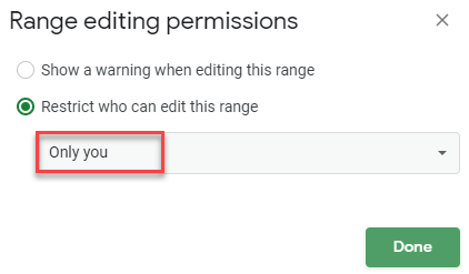
Now, only selected users can edit the range, while for all others, cells are locked for editing.

Note: To see, instead, how to lock a cell reference, see Freeze Cell in Formula or How to Anchor a Cell.