Lock / Freeze Cell in Formula in Excel & Google Sheets

This tutorial demonstrates how to lock a cell in a formula in Excel and Google Sheets.

 

 

Lock Cells in Formulas

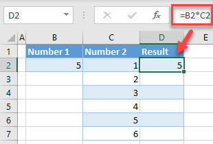
When you copy a formula, cell references in the formula change depending on where you paste. In some cases, you don’t want cell references to change and want to lock them when copying the formula. In the following example, Column D is the result of the multiplication of values from B2 and Column C.

 

 

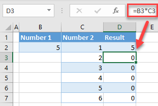
If you now copy the formula down Column D, both cell references change (B2 to B3 and C2 to C3, etc.).

 

 

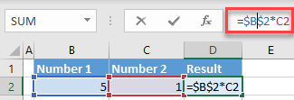
In this case, you don’t want B2 to change. To lock it, click on the cell reference in the formula bar (B2), and enter $ before column and row ($B$2). You can also press F4 on the keyboard to freeze a cell.

 

 

As a result, Column D now has cell B2 locked, and values from Column C are multiplied by 5 in every row.

 

 

Notes: In the newer version of Excel, there are new arrays formulas that automatically spill the values to the range, and don’t need any cell locking. These formulas are SORT, UNIQUE, SORTBY, XLOOKUP, etc.

To see, instead, how to lock a cell for editing, see How to Lock Cells.

Lock Cells in Google Sheets

You can use the same logic for locking cells in Google Sheets.