How to Unlock / Unprotect Cells in Excel & Google Sheets

In this tutorial, you will learn how to unlock cells in Excel and Google Sheets.

 

 

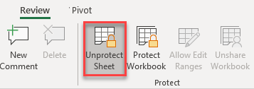
Unlock Cells

If you have a protected worksheet or range of cells, you can easily unlock it. (If the sheet is password-protected, you’ll need to provide the password to unlock it.) Say you have the following sheet with cells locked for editing and formatting.

 

 

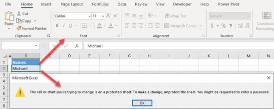
If you select cell C2, you can see that all formatting options in the Home tab are grayed out, which means you can’t format the cell. Also, if you try to edit the content of the cell, you get the message that it is locked for changes. To unlock the cells, follow these steps:

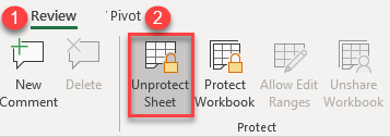
1. In the Ribbon, go to Review > Unprotect Sheet.

 

 

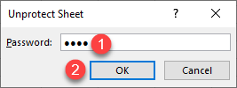
2. If the sheet is password-protected, in the pop-up window, enter a password, and click OK. (If the sheet is not password-protected, skip this step.)

 

 

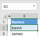
Cells are now unlocked, and you can change them (e.g., change cell B2 from “Michael” to “Kevin”).

 

 

If you need to lock the cells again, see How to Lock Cells or How to Password Protect a File.

Unlock Cells in Google Sheets

You can also unlock a range of cells or a sheet and enable changes in Google Sheets.

1. To see all protected ranges in Google Sheets, go to Data > Protected sheets and ranges.

 

 

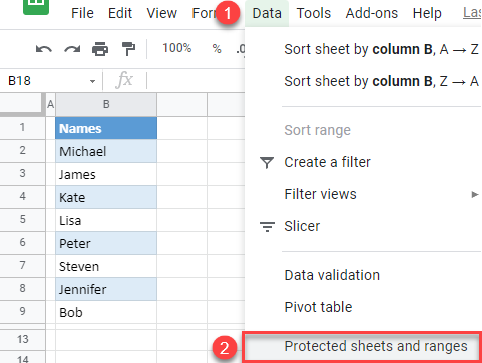
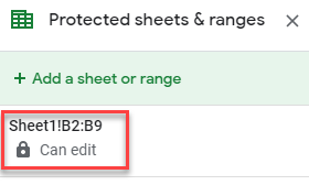
2. On the right side is the Protected sheets & ranges window. As you can see, the Sheet!B2:B9 range is protected. Click on it.

 

 

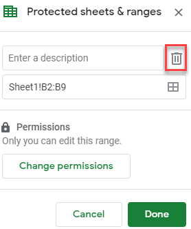
3. Click on the recycle bin icon to delete the protection from the range.

 

 

4. The pop-up warning is displayed, click Remove to confirm.

 

 

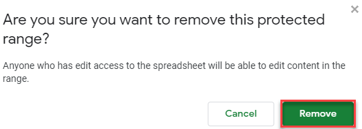
As a result, the range B2:B9 is now unlocked and enabled for editing.

Note: To see, instead, how to (un)lock a cell reference, see Freeze Cell in Formula or How to Anchor a Cell.