Hide / Unhide Rows or Columns in Excel & Google Sheets

In this tutorial, you will learn how to hide and unhide rows and columns in Excel and Google Sheets.

 

 

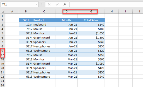
There are several ways to limit which rows and columns are visible in an Excel spreadsheet. This article will show how to use Hide and Unhide. Other options include VBA or Excel’s Outline feature.

Hide and Unhide Rows

Let’s start with the example below, a set of sales data, to show how to hide and unhide rows or columns.

 

 

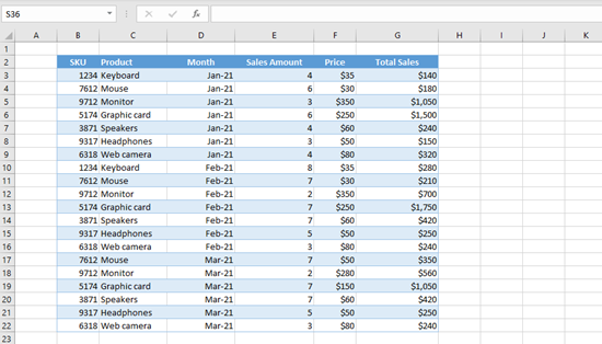
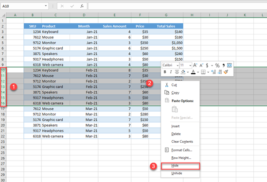
Let’s, for example, hide all rows for Feb-21 (10–16).

To do this, we need to select Rows 10 to 16, by (1) clicking and holding Row 10 heading and dragging until Row 16 (we can alternatively select Row 10, hold SHIFT, and select Row 16; this will select all rows between 10 and 16).

Then we need to (2) right-click anywhere in the selected area, and (3) click Hide.

 

 

As a result, Rows 10–16 are hidden, and we can’t see them in the worksheet.

 

 

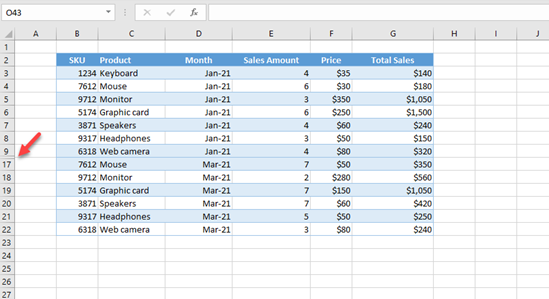
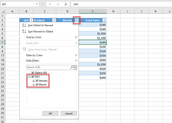
If we try to filter data by Month now (Column D), we’ll see that only values that are not hidden are displayed (Jan-21 and Mar-21) and Feb-21, which is hidden, is not shown.

 

 

Unhide Rows

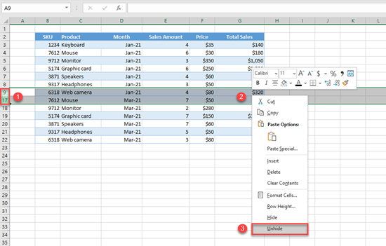
If we want to unhide these rows and display them again, first (1) select one row before and one row after the hidden rows (9 and 17). After that, we need to (2) right-click somewhere in the selected area, and (3) choose Unhide.

 

 

Now, Rows 10–16 are unhidden, and we can see them again.

Hide and Unhide Columns

Hiding and unhiding columns work like hiding rows. Only, instead of row numbers, we need to use column headings. Let’s say that we want to hide Sales Amount and Price from our sheet (Columns E and F). To do this, we need to select Columns E and F, by (1) clicking and holding Column E heading and dragging to Column F. Then we need to (2) right-click anywhere in the selected area, and (3) click Hide.

 

 

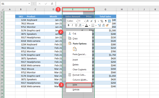
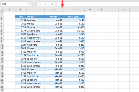
As a result, Columns E and F are hidden, and we can’t see them in the worksheet.

 

 

Unhide Columns

If we want to unhide these two columns and display them again, we need to do the following: First, we need to (1) select one column before and one column after the hidden columns (D and G). After that, we need to (2) right-click somewhere in the selected area, and (3) choose Unhide.

 

 

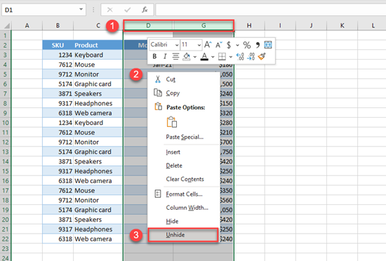
Finally, Columns E and F are unhidden, and we can see them again.

Hiding and Unhiding Rows and Columns in Google Sheets

Hiding and unhiding rows and columns work exactly the same in Google Sheets.