How to Group in Pivot Tables in Excel

This article will demonstrate how to group in pivot tables in Excel.

 

Group by Date in Excel Pivot Tables

Let us consider the data below:

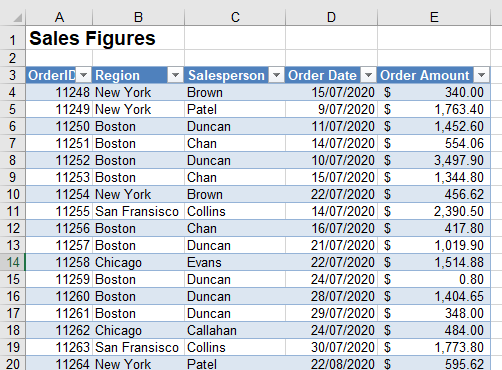
This sales data has 5 individual columns, and is made up of 800 rows of orders.   When we create a Pivot Table, we can select to add the Region to the Filter area, the Order Date to the row area and Order Amount to the value are of the Pivot table.

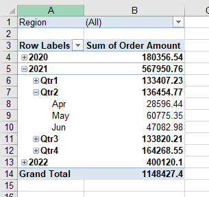
When we add a date to the filter, row or column areas of a pivot, the data will automatically be grouped by default into years and quarters.   Each group has an expand (+) icon attached to it.  If we click on this icon, it will change to a contract (-) icon.

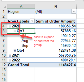
The row area of the Pivot fields will reflect that as well as the order date, the Quarters and Year fields have been created and added to the Pivot table.

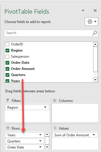
The date field itself has therefore been grouped by Year, Quarter and, Month.  You can remove any of these fields, but if we remove the Year for example, then the data will not  be divided into the individual years, e.g., all the orders for February will be included in Quarter1 > February regardless of what year the order is in.

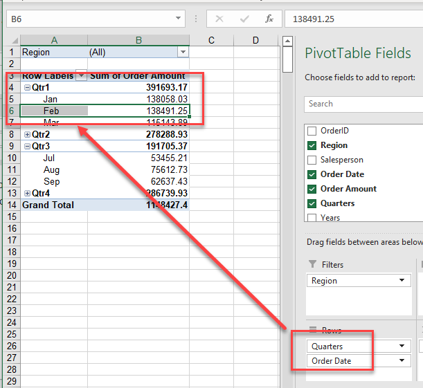
Similarly, if you remove the Quarters field, then only months will be shown – so all the orders in February, regardless of the year, will be shown in February.

 

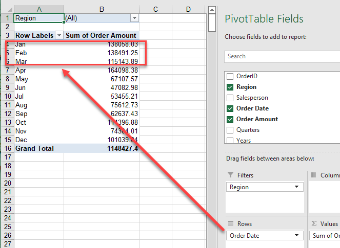
This is due to the fact that by default, the Pivot table does not group by individual dates.

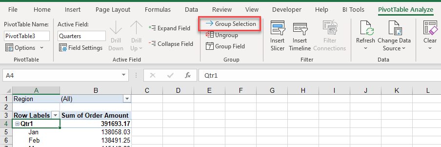
To amend the way that the Pivot table groups, select the row field in the Pivot table and then, in the Ribbon, select Pivot Table Analyze > Group > Group Selection.

 

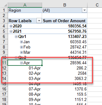
You can now add the actual date of the order (days) to the Pivot table as well.

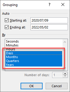
This enables you to drill down further and expand by Year, then by Quarter, then by Month to obtain the sales order amount for each individual day.

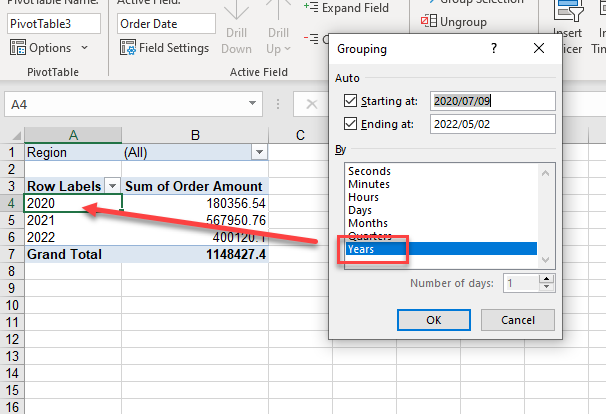
Similarly, you can remove the Months grouping and group just by Quarters and Years.

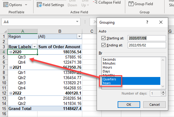
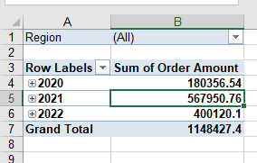
Or, remove both the Months and Quarters grouping and group just  by year.    This will just give you the order amounts for each year and will remove the ability to drill down to the individual quarters, months or dates.

Manual Grouping in Pivot Tables

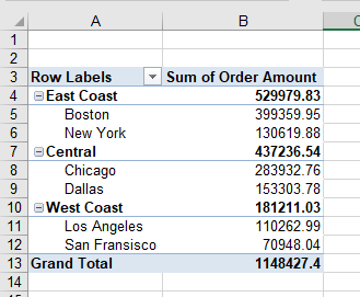
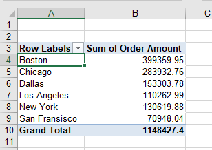
Let us consider the following Pivot table.

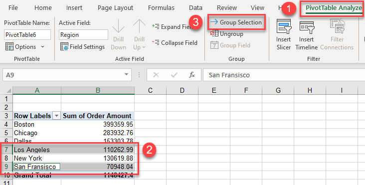
1. Click in the Ribbon and then select PivotTable Analyze.

2. Hold down the shift key, and select the field values  that you wish to group on.

3. In the Ribbon, select PivotTable Analyze > Group > Group Selection.

 

4. The values you selected will be grouped together.

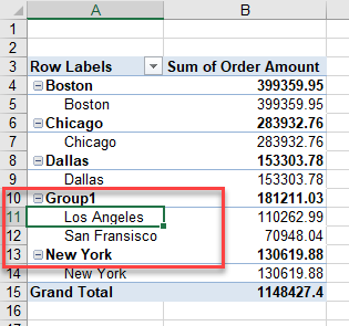
5. Click in the group name (eg Group 1) and type in a relevant name for your group.

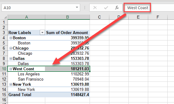
6. You can then select other values to group on, for example Boston and New York.  Remember to old down the shift key to select multiple values.  Once you have grouped your values together, you can rename the groups.