How to Create a Pivot Table in Excel & Google Sheets

This article will demonstrate how to create a Pivot Table in Excel & Google sheets.

 

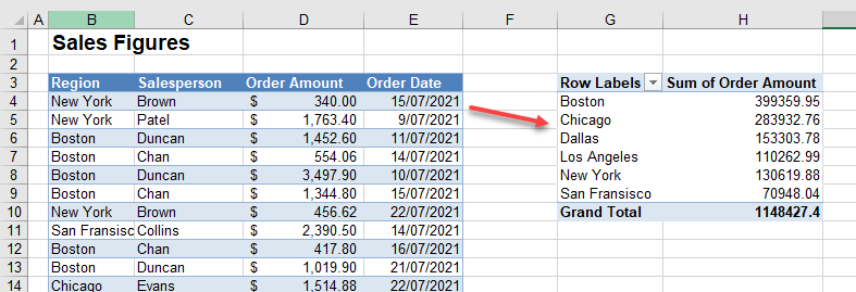
Create a Pivot Table

1. Make sure you clicked somewhere in the table of data that you wish to create a pivot table from.

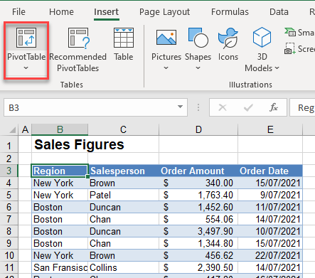
2. In the Ribbon, select Insert > Tables >Pivot Table.

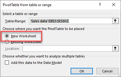
3. Select New Worksheet and then click OK.

 

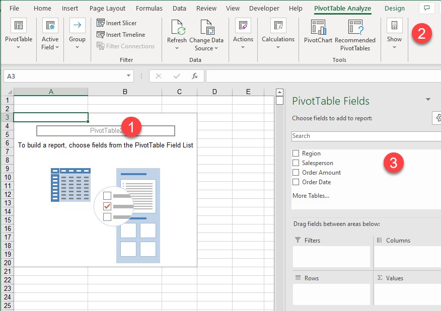
A new sheet will be created with a  (1) blank pivot table shown.   There are 2 new tabs added to the ribbon (2) – PivotTable Analyze and Design.    On the right hand side of the screen, (3) a task pane will appear with the Pivot table fields available.

 

4. Drag the fields down to the relevant sections of the pivot table.  In the example below, we have dragged the SalesPerson to the Filter section, the Region to the Rows section and the Order Amount to the values section.

 

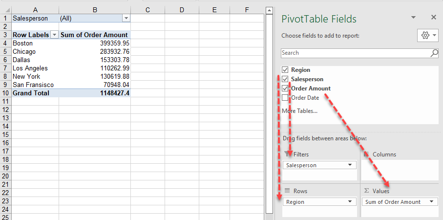
You can play around with the fields and drag them betwen Rows, Columns and Filters.  Note that anything dragged to the Values that is not a number will automatically be counted rather than summed!

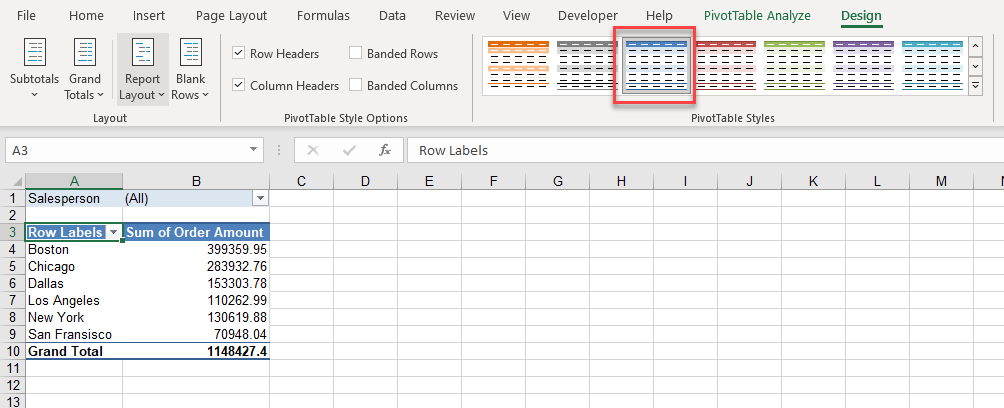
5. If you wish to change the format of the Pivot table, you use the Design tab to do this.    Select PivotTable Styles and select the style you require.  This will format the pivot table in a similar way to the Excel function “Format as a Table”

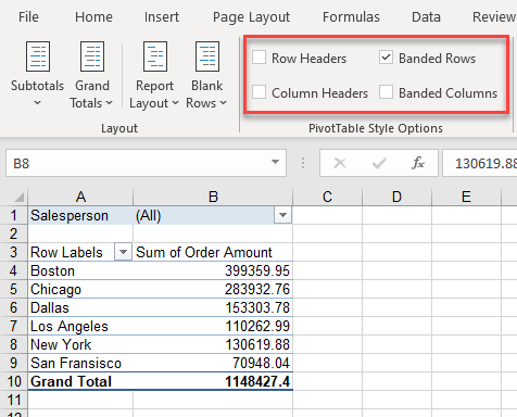
6. To amend a selected style, we can select from the options in the PivotTable Style Options group – for example Row Headers, Column Headers, Banded Columns and Banded Rows can either be selected to be shown, or de-selected to no be shown in the Pivot table.

 

To clear the formating, you can select Clear at the bottom of the drop down of Pivot table Styles.

 

 

Refresh a Pivot Table

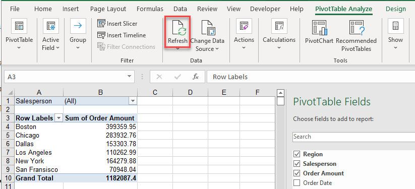
If your underlying data changes, you will need to refresh your pivot table to update the values.

In the Ribbon, select PivotTable Analyze > Data > Refresh.

Delete a Pivot Table

In the Ribbon, select PivotTable Analyze > Actions > Select All.

 

Press the Delete key to delete the Pivot table.  Note that this will only delete the Pivot table and not the underlying data that the Pivot table relies on.

Filter and Sort in a Pivot Table

When you create a Pivot table, a drop down filter is automatically created on the row or column labels, as well as any field that you may have selected to be the filter field at the top of the Pivot table.  This filter is similar to the usual Filter function in Excel.

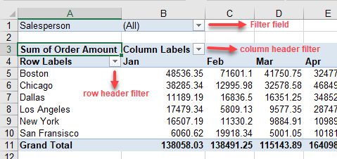
1. To filter a pivot table, select any of the drop down filters, and then select the filter required.

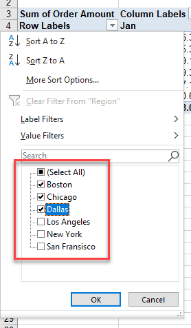
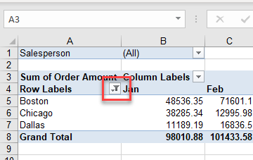
2. Click OK to show the selected filtered data.  You will notice that any of the filter drop downs that has a filter applied will show a little ‘funnel’ icon indicating that not all the data is being displayed.

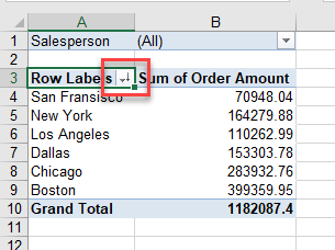
3. When you click on the drop down arrow for to filter the data, instead of filtering the data, you might like to sort the data.   Sorting data in a Pivot table works in the same way as sorting data in an Excel worksheet.

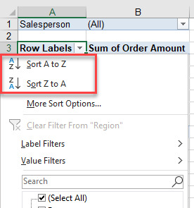
4. Click on Sort Z to A to reverse the order of the data.  You will notice once you have done this that  little arrow in the direction of the sort will appear on the filter button.

Grouping in a Pivot Table

Grouping like rows or columns together is an often used feature in Excel.  Grouping can also occur in Pivot tables when you either add 2 of more fields to the Row and / or column sections; or if you add a date or numeric field to the row and / or column section.

1. Add 2 fields to the rows section to add grouping to the Pivot table.

 

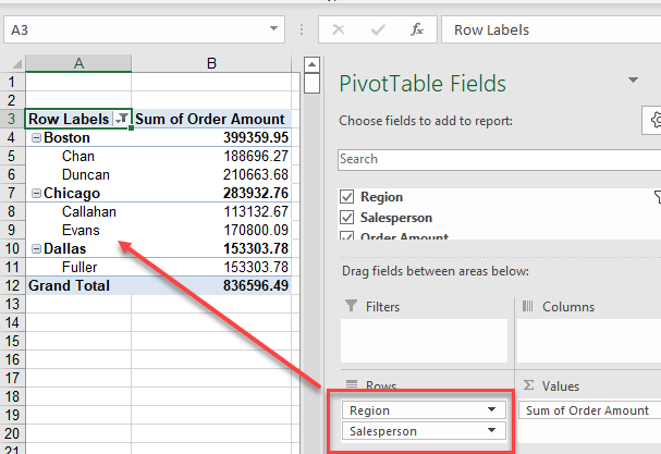
If the Row or Column field is a date or numeric, then the Group section in the PivotTable Analyze tab of the Ribbon will become available.

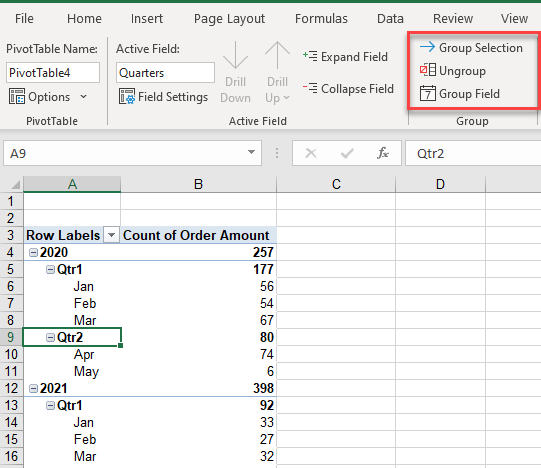
2. Click on Group Selection.

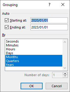
3. As a date field is the row field, it has already been grouped into Months, Quarters and Years.  To remove the Quarters group, click on the Quarter to de-select it, and then click OK.

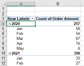
4. To remove all the grouping, select Ungroup.

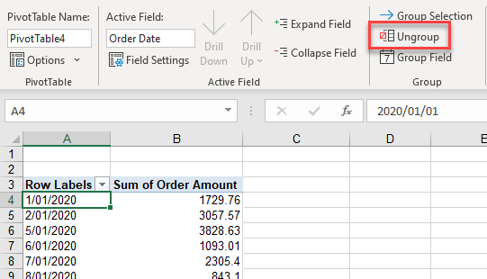
5. Select Group Selection or Group Field to regroup the data if required.

Create a Pivot Chart

1. To create a chart based on your Pivot table, click within the Pivot table and then, in the Ribbon, select PivotTable Analyze > Tools > PivotChart.

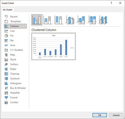
2. Select the type of chart you want, and then click OK.

 

You will notice that (1) the PivotTable Analyze tab on the ribbon is now replaced with the PivotChart Analyze tab.   The chart is the same as any other Excel chart that you may have created except for the fact that it has (2) filter available on the fields that can be filtered in your Pivot table.  For example, in the chart below we can filter on the Salesperson and Region.

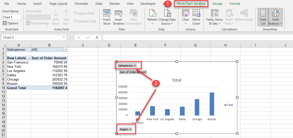
The Design tab is much the same as the design tab when creating a normal Excel chart in that it enables you to customize the chart by changing the chart type, adding elements or changing the chart colors.

How to Create a Pivot Table in Google sheets

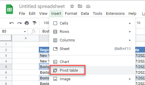
1. Click in the table of data from which you wish to create your pivot table, and then, in the Menu, select Insert > Pivot table.

 

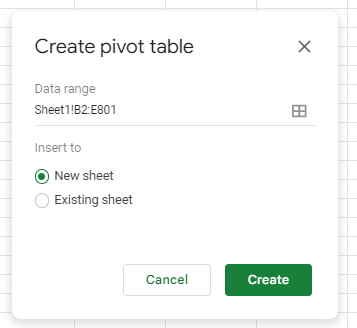
2. Select Insert to New Sheet and click Create.

 

3. From the task pane on the right hand side of your screen, select the fields to add to the rows, columns and values section of your Pivot Table. This is much the same as Excel.

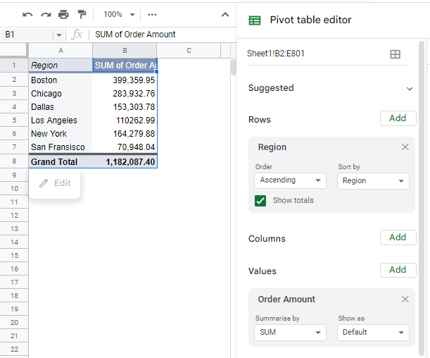
4.  A Pivot table in Google Sheets will automatically refresh if the data changes – it does not need to be manually refreshed.

The sorting and grouping options that are available in Excel Pivot tables are not available in a Google sheets Pivot table, however the ability to filter the data is.

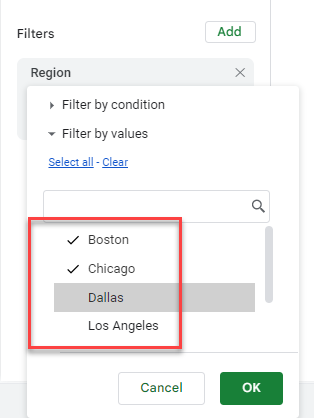
5. To create a filter, you need to add a filter.  In the filters section, click the Add button and select the field to filter on.

 

 

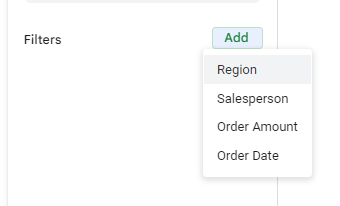
5. Select the data you wish to show in the Pivot table filter, and then click OK.

To delete a Pivot table in Google Sheets, select all the columns and rows of the Pivot table and press Delet