Show or Hide AutoFilter Arrows in Excel & Google Sheets

This tutorial demonstrates how to show or hide AutoFilter arrows in Excel and Google Sheets.

 

 

Show AutoFilter Arrows

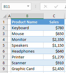
Whenever you filter data in Excel, filter arrows appear in the heading of your data range. Say that you have the following data set with Product Name in column B and Sales in column C.

 

 

When you want to display AutoFilter arrows in order to be able to filter data, you have to (1) click anywhere in the data range (in this example, B1:C9), and in the Ribbon, (2) go to Home > Sort & Filter > Filter.

 

 

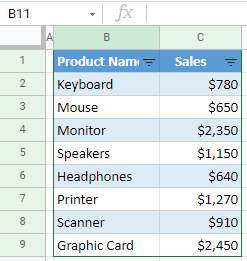
As a result, AutoFilter arrows are now displayed in the header data (row 1) next to Product Name and Sales.

 

 

Now, let’s say that you want to filter data, for example, show only products that have sales greater than $1,000. To do this, (1) click on the filter arrow next to Sales (cell C1), (2) select Number Filters, and (3) choose Greater Than…

 

 

In the pop-up window, by default is greater than is selected, so (1) enter 1000, and (2) click OK.

 

 

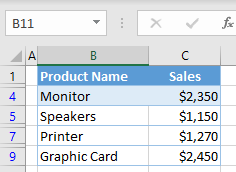
As a result, only rows with Sales in column C greater than $1,000 are displayed (rows 4, 5, 7, and 9 – highlighted in blue).

 

 

As you can see, AutoFilter arrows in the header row are still displayed. In the next section, you will find out how to hide these arrows.

Hide AutoFilter Arrows

In order to filter data and hide AutoFilter arrows, you have to use an advanced filter. Let’s use the same example with product name and sales. You have to add a criteria value in form of a table with the same heading name (Sales) and criteria value (>1000) somewhere out of the filtering range. In this example, the criteria range is E1:E2.

 

 

To filter and hide AutoFilter Arrows, follow the next steps.

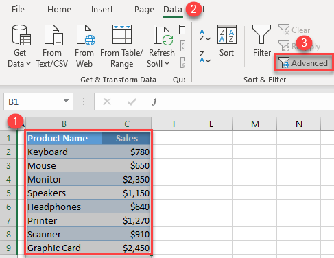
1. Select the range you want to filter (in this example B1:C9), and in the Ribbon, (2) go to Data > Advanced (in the Sort & Filter group).

 

 

2. In the pop-up window, select the criteria range (in this example range E1:E2), and press OK.

 

 

As a result, data are filtered just like in the previous section, but now AutoFilter arrows are hidden.

 

 

Show AutoFilter Arrows in Google Sheets

In order to add AutoFilter arrows in Google Sheets, (1) click anywhere in the data set, and (2) click on the Create a filter icon in the menu.

 

 

As a result, AutoFilter arrows are added to the header, and you can filter your data.

 

 

Unfortunately, in Google Sheets, you can’t hide AutoFilter arrows once you filter data.