How to Sort by Last Name in Excel & Google Sheets

In this tutorial, you will learn how to sort names by last name in Excel and Google Sheets.

 

 

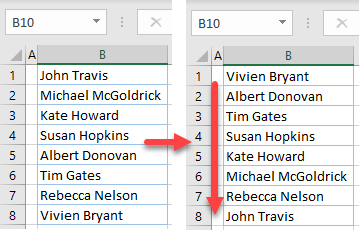
Assuming you have a first and last name together in one cell, there are several different ways to extract the last name and sort the full name column by last name.

Sort by Last Name

Sort With Text to Columns

The first option to sort by last name is to extract the last name from the full name in a separate column using the text to columns feature in Excel. Say you have the following list of names, containing only one first name and one surname separated by a space, in Column B:

 

 

1. Select the column you want to sort (B in this example), and in the Ribbon, go to Data > Text to Columns.

 

 

2. In the Convert Text to Columns Wizard, Step 1, leave Delimited checked, and click Next.

 

 

3. On the Step 2 screen, check Space and click Next.

 

 

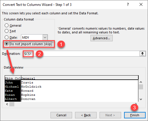
4. For Step 3, select Do not import column (skip) under Column data format. In the Destination, enter the cell where you want the extracted data to go (in this case $C$1) and click Finish.
   This means you will skip the first column (first name), as you don’t need it, and get only the second column extracted (last name) in Column C, starting from cell C1.

 

 

5. Now you have last names in Column C next to the full names in Column B, and you can sort both columns by Column C.
   To do that, select the column with last names and in the Ribbon, go to Home > Sort & Filter > Sort A to Z.

 

 

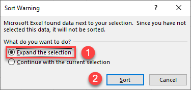
6. In the pop-up warning, leave Expand the selection checked and click Sort. This means that you want all populated columns (B and C) to be sorted based on Column C.

 

 

After the sort is done, all values in Column B are sorted alphabetically by last name, and you can delete Column C, as you don’t need it anymore.

 

 

Sort With Flash Fill

The second option to achieve the same result is to use Flash Fill. This option recognizes patterns by two or more entries.

1. Enter the first two last names in cells C1 and C2 (Travis and McGoldrick) and select them. Now position the cursor in the bottom right corner of the selection area, until it turns into a cross and double-click it.

 

 

2. Click on the AutoFill options button that appears at the end of the selection and choose Flash Fill.

 

 

As you can see, Excel automatically recognizes that you want to extract last names based on the space in Column B and populates the rest of Column C automatically. Now you can sort the range the same way as in the section above.

Sort With Find and Replace

Another way to sort by last name is to use Find and Replace.

1. Select Column B and copy it (CTRL + C), then select cell C1 and paste the copied column (CTRL + V).

 

 

2. Select Column C, and in the Ribbon go to Home > Find & Select > Replace (or use the keyboard shortcut, CTRL + H).

 

 

3. In the pop-up window enter an asterisk and a space (* ) in Find what, leave Replace with blank, and click Replace All.
   In Find, an asterisk represents any character, so when you put asterisk-space in Find, Excel will find all characters before a space and replace them with an empty value (delete them).

 

 

As a result, all first names and spaces are now removed from each cell. Only the last names are in Column C. After this, you can sort the column the same way as in the section above.

 

 

Another option is to use VBA code to sort data by last name.

Sort by Last Name in Google Sheets

Since Google Sheets doesn’t have options like Excel’s Flash Fill and Text to Columns, you can use functions to create a formula that will extract the last name in Column C. The same formula can also be used in Excel with the same syntax.

1. Select cell C1, and enter the formula:

=RIGHT(B1,LEN(B1)-FIND(" ",B1))

 

 

• • The LEN Function finds the length of text in cell B1 (which is 11).
  • The FIND Function returns the position of the text you’re searching for (space) in cell B1 (which is 5).
  • The RIGHT Function returns the specified numbers of characters (11–5 = 6) from the end, in the given cell (B1).

As the final result, you get the last six characters from B1, which is the last name (Travis).

2. Position the cursor in the bottom right corner of cell C2 until the cross appears.

 

 

3. Drag the formula down to the end of the range (C8).

 

 

4. When you have all last names extracted, you can sort the data in Column B.
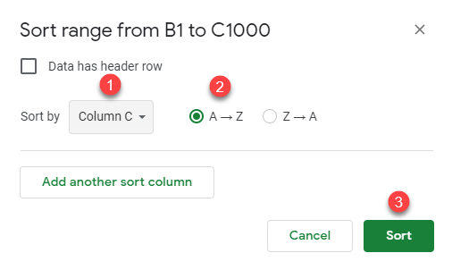
   Select Columns B and C, and in the Menu, go to Data > Sort range.

 

 

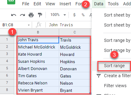
5. In the pop-up window, select Column C and A → Z under Sort by, and click Sort.

 

 

Now, you can delete Column C, as the names in Column B are sorted by last name alphabetically, from A to Z.