How to Sort and Ignore Blanks in Excel & Google Sheets
In this tutorial, you will learn how to sort while ignoring blanks in Excel and Google Sheets.
Sort and Ignore Blanks
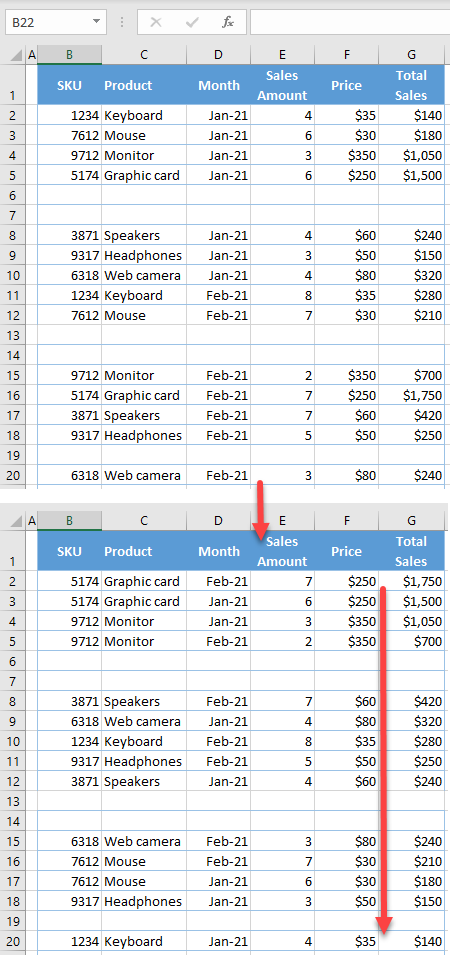
Sometimes in Excel, you’ll want to sort a data range that has blank rows. If you simply sort the data, Excel will automatically push blank rows to the very end. Look at the following data set to see how to ignore blanks when sorting data so the blank rows remain where they were before sorting.
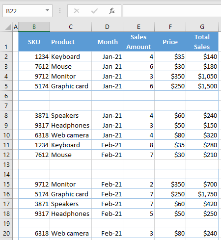
In this example, you have blank rows (6, 7, 13, 14, and 19). You want to sort the data by Total Sales from largest to smallest and ignore blanks.
- Select rows that you want to hide (6 and 7), right-click anywhere in the selected area and click Hide.

- Repeat Step 1 for Rows 13 and 14, then for Row 19. Now the five blank rows are hidden, and the data range looks like this:

- Right-click anywhere in the selected area and click Hide. The result is the same as in the previous steps: All blank rows are hidden.
- Now you can sort the data range by Total Sales and Excel will ignore the blank rows. To do this, select Column G then in the Ribbon, go to Home > Sort & Filter > Sort Largest to Smallest.

- In the pop-up window, choose Expand the selection and click Sort.

As a result of this step, the data range is sorted by Total Sales in descending order, but blank rows are still hidden.

- Finally, unhide all blank rows (6, 7, 13, 14, and 19).
Select all rows in the data range (1:20), right-click anywhere in the selected area and click Unhide.
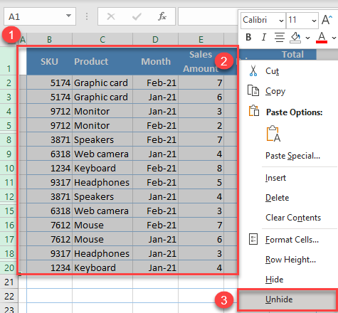
Now, you have data sorted by Total Sales. Blank rows were ignored, and they remain where they initially were.

Hide All Blank Rows at Once
There is another way to hide rows that allows you to hide all blank rows at once.
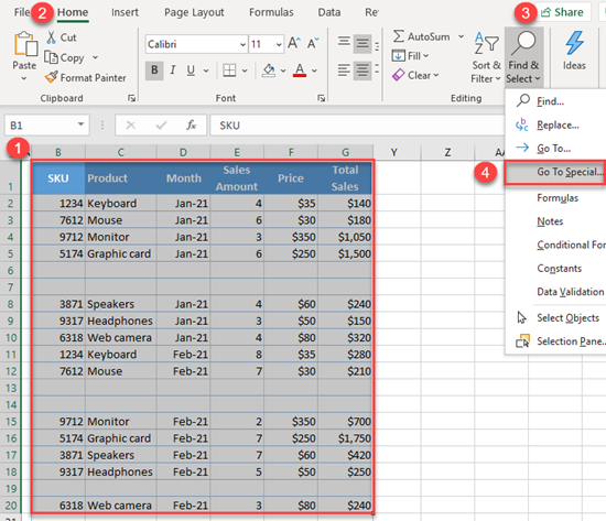
- Select the data range (B1:G20), and in the Ribbon, go to Home > Find & Select > Go To Special…
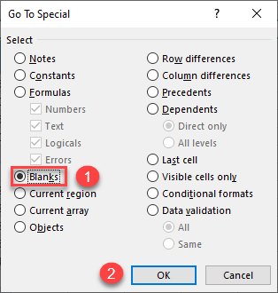
- In the pop-up window, select Blanks and click OK.
- Continue with Steps 3–6 above.
All blank cells in the data range are selected.

Sort and Ignore Blanks in Google Sheets
In Google Sheets, performing a sort with blanks ignored is done a bit differently.
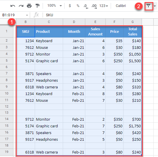
- Select the data range (B1:G20) and click on the Filter icon in the toolbar.
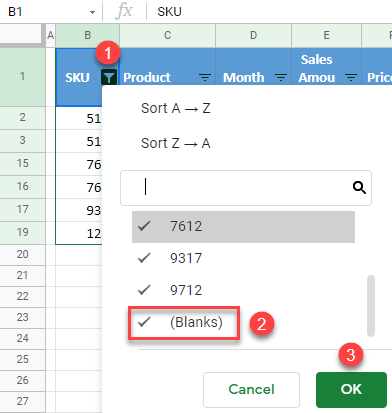
- Click on the filter button next to SKU (cell B1), uncheck (Blanks), and click OK.

- Now, all blank rows are hidden, and you can sort the data range.
Click on the filter button next to Total Sales (cell G1) and choose Sort Z → A (descending).

- The data range is now sorted by Total Sales in descending order, and you can unhide blank rows.
Click on the filter button next to SKU (B1), check (Blanks), and click OK.
Finally, all rows are visible, and the data range is sorted ignoring the blank rows.
