Highlight Every Other Line In Excel – Excel & Google Sheets

This tutorial will demonstrate how to highlight every other row using Conditional Formatting and Table formatting in Excel and Google Sheets.

Highlight Every Other Line

To highlight every other row with Conditional Formatting, use the ISEVEN or MOD Functions within a Conditional Formatting rule.

1. Select the range you want to apply formatting to.
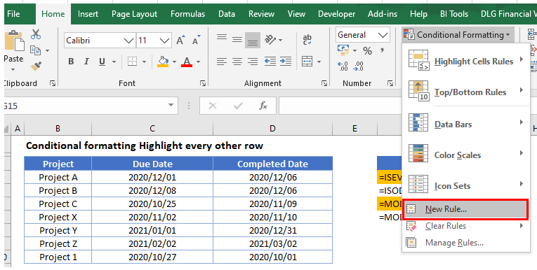
2. In the Ribbon, select Home > Conditional Formatting > New Rule.

3. Select “Use a formula to determine which cells to format‘, and enter the following formula (with the ROW Function):

=ISEVEN(ROW())

OR

=MOD(ROW(),2)=1

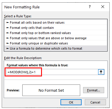
4. Click on the Format button and select your desired formatting.

5. Click OK, and then OK again to view the result.

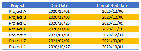
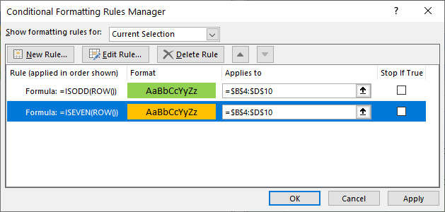
You can apply a similar rule using the ISODD formula =ISODD(ROW()) or =MOD(ROW(),2)=0 to highlight all the odd rows in the table.

OR

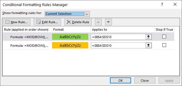
The result will then be:

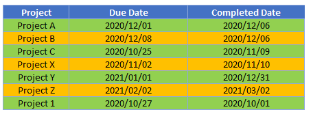
Where all the even rows are green and all the odd rows are orange.

Excel Tables

You can also highlight every other row in Excel by using the table formatting option.

1. Select the range you wish to highlight.
2. Click on Home>Format as Table.

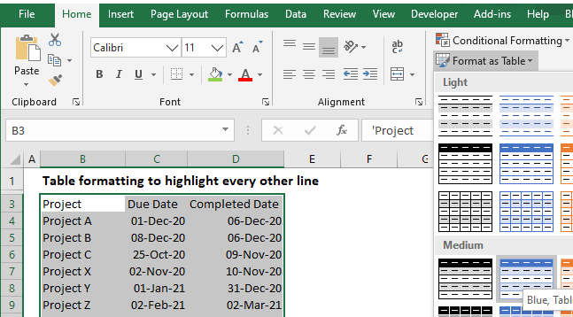
3. Select the type of formatting you require.

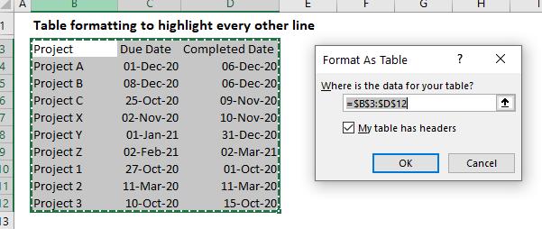
4. Check if your table has a header row, and if so, keep the check box ticked, and click OK.

5. The table is formatted including a filter row at the top. To remove the filter row and convert your table to a standard range, click in your table, and then click Convert to Range in the Tools section of the Design tab of your toolbar.

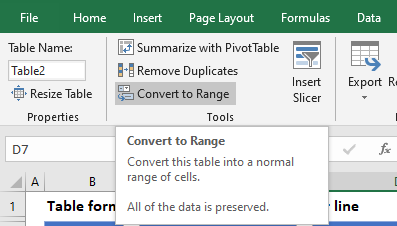
6. A warning box will appear. Select Yes to convert the table to a normal range.

7. Your format will then be applied but the Design toolbar will no longer appear when you click in your table.

Highlight Every Other Line in Google Sheets

The process to highlight odd and even rows in Google Sheets is similar to the process in Excel.

1. Highlight the cells you wish to format, and then click on Format > Conditional Formatting.

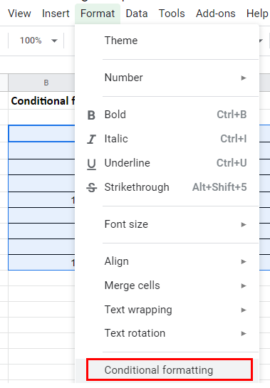
2. The Apply to Range section will already be filled in.

3. From the Format Rules section, select Custom Formula from the drop-down list and type in the following formula:

=ISEVEN(ROWS())

4. Select the fill style for the cells that meet the criteria.

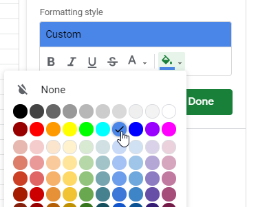
5. Click Done to apply the rule.

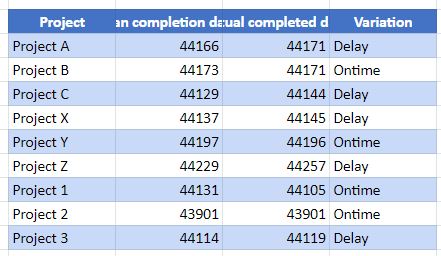
6. Click Add another rule to add a rule for the odd rows.

7. Select Custom Function and type in the formula.

=ISODD(ROWS())

8. Click Done to apply the rule.

You can also use the =MOD(ROW(),2)= 1 and =MOD(ROW(),2=0 to achieve the same result.