Find and Extract Number from String – Excel & Google Sheets

This tutorial will demonstrate you how to find and extract a number from inside a text string in Excel and Google Sheets.

Find and Extract Number from String

Sometimes your data may contain numbers and text and you want to extract the numerical data.

If the number part is on the right or left side of the string, it’s relatively easy to split the number and text . However, if the numbers are inside the string, i.e. between two text strings, you will need to use a much more complicated formula (shown below).

TEXTJOIN – Extract Numbers in Excel 2016+

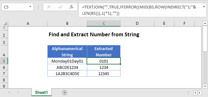
In Excel 2016 the TEXTJOIN function was introduced, which can extract the numbers from anywhere of the text string. Here is the formula:

=TEXTJOIN("",TRUE,IFERROR((MID(B3,ROW(INDIRECT("1:"&LEN(B3))),1)*1),""))

Let’s see how this formula works.

The ROW, INDIRECT and LEN Functions returns an array of numbers corresponding to each character in your alphanumerical string. In our case, “Monday01Day” has 11 characters, so the ROW function will then return the array {1;2;3;4;5;6;7;8;9;10;11}.

=TEXTJOIN("",TRUE,IFERROR((MID(B3, {1;2;3;4;5;6;7;8;9;10;11},1)*1),""))

Next, the MID Function extracts each character from the text string, creating an array containing your original string:

=TEXTJOIN("",TRUE,IFERROR(({"M";"o";"n";"d";"a";"y";"0";"1";"D";"a";"y"}*1),""))

Multiplying each value in the array by 1 will create an array containing errors If the array character was text:

=TEXTJOIN("",TRUE,IFERROR(({#VALUE!;#VALUE!;#VALUE!;#VALUE!;#VALUE!;#VALUE!;0;1;#VALUE!;#VALUE!;#VALUE!}),""))

Next, the IFERROR Function, removes the error values:

=TEXTJOIN("",TRUE,{"";"";"";"";"";"";0;1;"";"";""})

Leaving only the TEXTJOIN Function which joins the remaining numbers together.

Note that the formula will give you all the numeric characters together from your string. For example, if your alphanumerical string is Monday01Day01, it will give you 0101 as a result.

Extract Numbers – Before Excel 2016

Before Excel 2016, you could use a much more complicated method to extract numbers from text. You can use the FIND function together with the IFERROR and MIN functions to determine both the first position of the number part and the first position of the text part after the number. Then we simply extract the number part with the MID function.

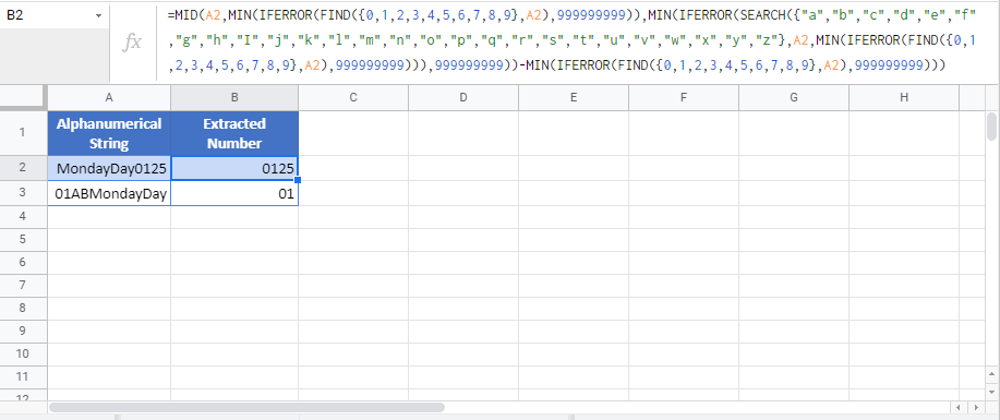
=MID(B3,MIN(IFERROR(FIND({0,1,2,3,4,5,6,7,8,9},B3),999999999)),MIN(IFERROR(SEARCH({"a","b","c","d","e","f","g","h","I","j","k","l","m","n","o","p","q","r","s","t","u","v","w","x","y","z"},B3,MIN(IFERROR(FIND({0,1,2,3,4,5,6,7,8,9},B3),999999999))),999999999))-MIN(IFERROR(FIND({0,1,2,3,4,5,6,7,8,9},B3),999999999)))

Note: This is an Array formula, you must enter the formula by pressing CTRL + SHIFT + ENTER, instead of just ENTER.

Let’s see step by step how this formula works.

Find Fist Number

We can use the FIND function to locate the starting position of the number.

= MIN(IFERROR(FIND({1,2,3,4,5,6,7,8,9,0},B3),999999999))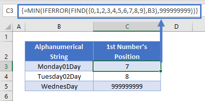

For the find_text argument of the FIND function, we use the array constant {0,1,2,3,4,5,6,7,8,9}, which makes the FIND function to perform a separate search for each value in the array constant.

The within_text argument of the FIND function in our case is Monday01Day, in which 1 can be found at the position 8, and 0 at the position 7, so our result array will be: {8,#VALUE,#VALUE,#VALUE,#VALUE,#VALUE,#VALUE, #VALUE, #VALUE,7}.

Using the IFERROR function we replace the #VALUE errors by 999999999. Then we simply look for the minimum within this array and get therefore the place of the first number (7).

Please note that the above formula is an array formula, you have to press Ctrl+Shift+Enter to trigger it.

Find First Text Character After Number

Similarly to locating the first number within the string, we use the FIND function to determine where the text begins again after the number making good use also of the start_num argument of the function.

=MIN(IFERROR(FIND({"a","b","c","d","e","f","g","h","I","j","k","l","m","n","o","p","q","r","s","t","u","v","w","x","y","z"},B3,C3),999999999))

This formula works very similarly to the previous one used for locating the first number, only we use letters in our array constant and therefore numbers cause #VALUE errors. Please note that we start searching only after the position determined for the first number (this will be the start_num argument) and not from the beginning of the string.

Don’t forget to press Ctrl+Shift+Enter to use of the above formula.

There is nothing left than putting this all together.

Extract Number From Two Texts

Once we have the starting position of the number part and the beginning of the text part after that, we simply use the MID function to extract the desired number part.

=MID(B3,C3,D3-C3)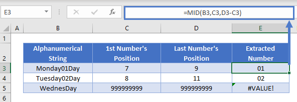

Other Method

Without explaining it in more detail, you can also use the below complex formula to get the number from inside a string.

=SUMPRODUCT(MID(0&B3,LARGE(INDEX(ISNUMBER(--MID(B3,ROW(INDIRECT("1:"&LEN(B3))),1))*ROW(INDIRECT("1:"&LEN(B3))),0),ROW(INDIRECT("1:"&LEN(B3))))+1,1)*10^ROW(INDIRECT("1:"&LEN(B3)))/10)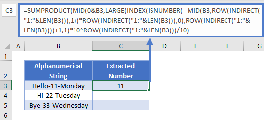

Please be aware that this formula above will give you 0 when there is no number found in the string and that leading zeros will be left out.

 

Find and Extract Number from String to Text in Google Sheets

The examples shown above work the same way in Google Sheets as they do in Excel.