VLOOKUP – Dynamic Column Reference – Excel & Google Sheets

This tutorial will demonstrate how to perform a VLOOKUP with a dynamic column references using the VLOOKUP and MATCH Functions in Excel and Google Sheets. If you have access to the XLOOKUP Function, we recommend using a Dynamic XLOOKUP instead.

VLOOKUP Row and Column Coordinates

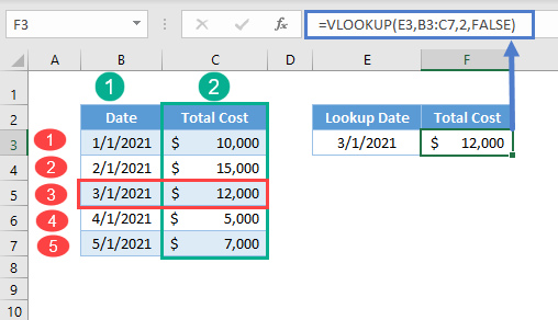
In general, all lookup processes require at least two things: the row and column coordinates of the value that will be looked up. With VLOOKUP, the row coordinate is determined by finding the lookup_value in the table_array. The col_index (3^rd argument) provides column coordinate.

VLOOKUP with Match Function

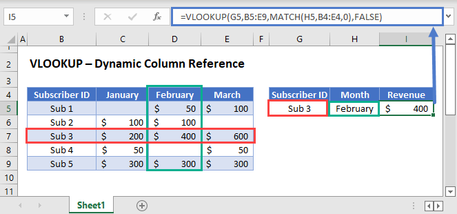
Typically, we use the VLOOKUP Function with a constant column index number (as shown above). Instead, we can use a MATCH Function to calculate the column number.

=VLOOKUP(G3,B3:E7,MATCH(H3,B2:E2,0),FALSE)

Let’s walkthrough the formula:

Match Function

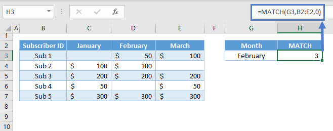
First, use the MATCH Function to look up the correct column number.

=MATCH(G3,B2:E2,0)

Here we look up “February” in row 2 and find that “February” is found in the 3rd column of the table.

VLOOKUP Function

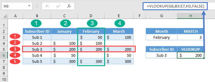
Next, we’ll use the result of the MATCH Function as the input for the column index of the VLOOKUP Function:

Putting this all together, we get our original formula:

=VLOOKUP(G3,B3:E7,MATCH(H3,B2:E2,0),FALSE)

In summary, the formula performs two lookups, which are in vertical and horizontal directions: one from VLOOKUP (vertical lookup) and another from the MATCH Function (horizontal lookup); hence, it’s called a two-way lookup. An alternative to this formula is the INDEX-MATCH-MATCH combination.

 

VLOOKUP-MATCH in Google Sheets

The VLOOKUP-MATCH formula works the same way in Google Sheets.