Insert and Remove Page Breaks in Excel & Google Sheets

This tutorial demonstrates how to insert and remove page breaks in Excel and Google Sheets.

 

 

Insert Page Breaks

In Excel, you can choose when to go to the next page when printing by setting page breaks. Let’s look at the following example and see how to insert a page break.

 

 

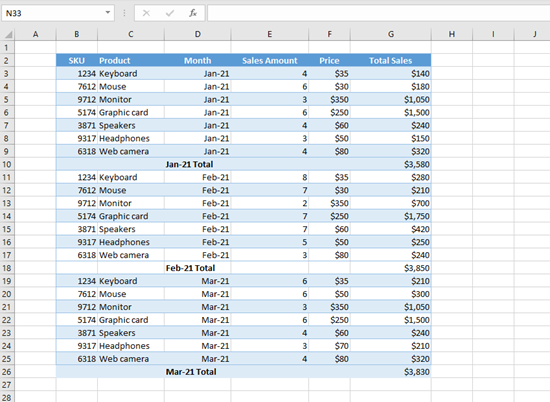
In this table, there’s sales data with subtotals, grouped by month. Say you want to print data for every month on a separate page. Insert page breaks after Jan-21 Total, Feb-21 Total, and Mar-21 Total.

1. First select the row right below where you want to insert a page break. In this case, select Row 11, since you want to insert a page break after Row 10.
2. After that, go to the Page Layout tab in the Ribbon, then click on Breaks in the Page Setup group, and choose Insert Page Break.

 

 

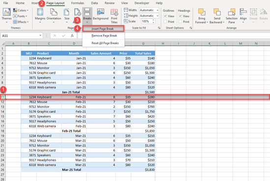
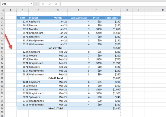
As a result, you get the page break line between Rows 10 and 11.

 

 

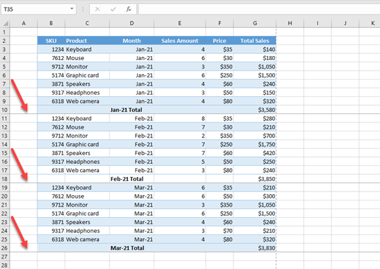
3. Now repeat steps 1 and 2 for Rows 19 and 26. Finally, you get two more page breaks between Rows 18 and 19, and then Rows 25 and 26.

 

 

Page Break Preview and Adjust

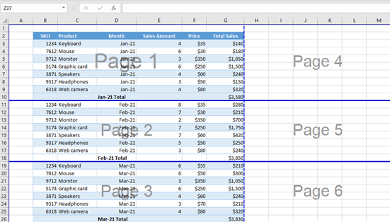
You can also display all page breaks in the sheet. Go to the View tab in the Ribbon and click on Page Break Preview.

 

 

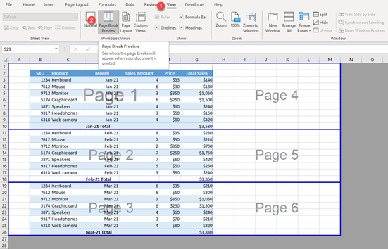
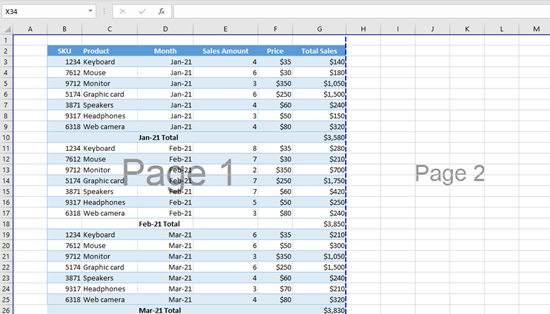
Here, you can see all page breaks and enumerated pages for printing. You can also adjust the page break by dragging it up or down. For example, if you want to have just one page for all rows, you need to drag the first page break to Row 27. Position the cursor on a page break line (between Rows 10 and 11) until the double arrow appears and drag the arrow down to Row 27.

 

 

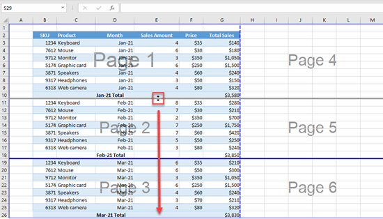
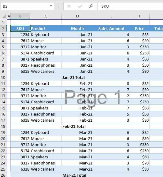
The page break is moved through to the end of the table, and all data will print on one page, as shown in the picture below.

 

 

Remove Page Breaks

1. To remove a page break, first go to the View tab in the Ribbon, and click on Page Break Preview.

 

 

2. Select the row above the page break you want to delete. In this case, select Row 11, as you want to delete the page break after Row 10.
3. After that, go to the Page Layout tab in the Ribbon, then click on Breaks in the Page Setup group, and choose Remove Page Break.

 

 

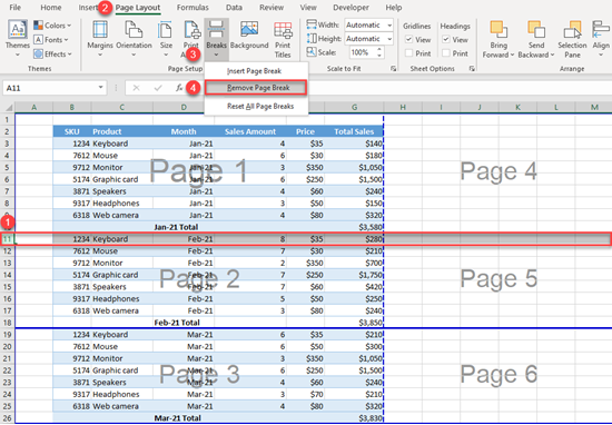
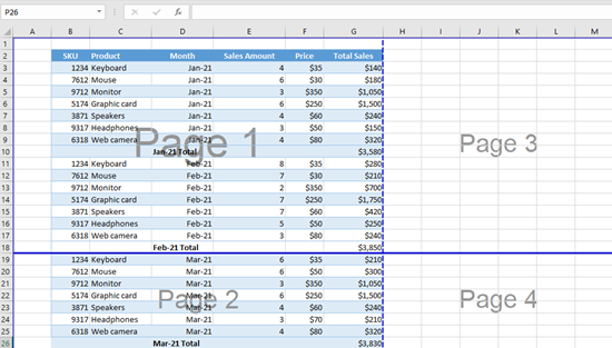
As a result, the first page break is removed and you now have two pages for printing, instead of three.

 

 

Remove All Page Breaks

You can also remove all page breaks at once. First, go to the Page Layout tab in the Ribbon, then click on Breaks in the Page Setup group, and choose Reset All Page Breaks.

 

 

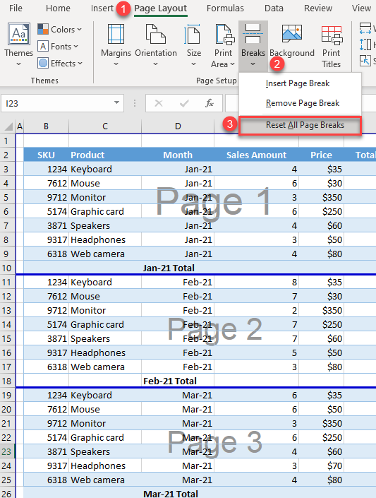
Now, all the page breaks are cleared and all data will print on one page.

 

 

Insert Page Breaks in Google Sheets

You can also insert custom page breaks in Google Sheets, but it’s a bit different compared to Excel. Say you have the same data set and want to set similar page breaks after each month subtotal.

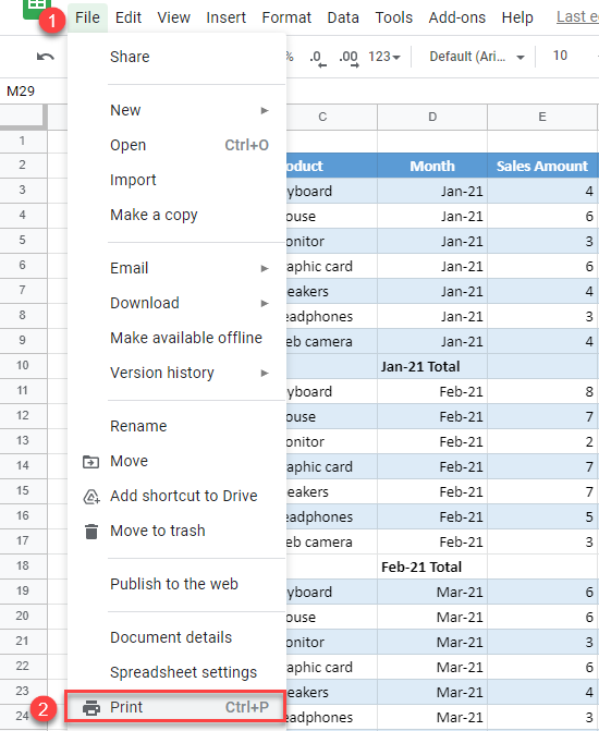
1. First, go to the File tab in the menu and click on Print (or use the keyboard shortcut CTRL + P).

 

 

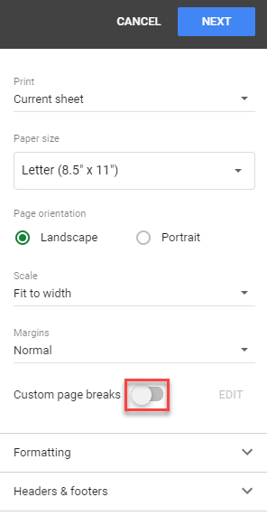
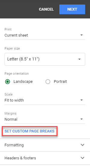
2. In the Print settings screen, go to Set Custom Page Breaks.

 

 

3. In the next screen, position the cursor at the bottom of the print area until the double-sided arrow appears. Then click and drag the arrow between Rows 10 and 11.

 

 

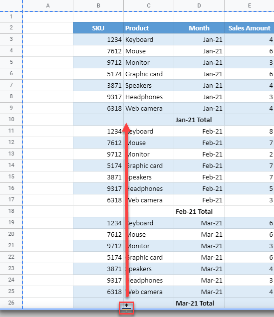
4. As a result, a page break appears between Rows 10 and 11. Click Confirm Breaks in the top right corner of the screen.

 

 

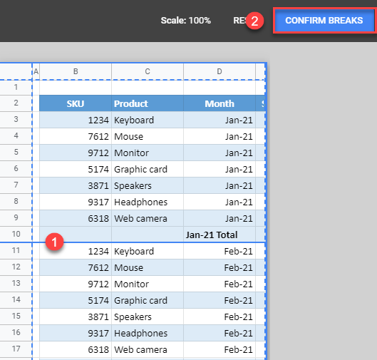
5. Now repeat the previous steps to insert the second page break between Rows 18 and 19.

 

 

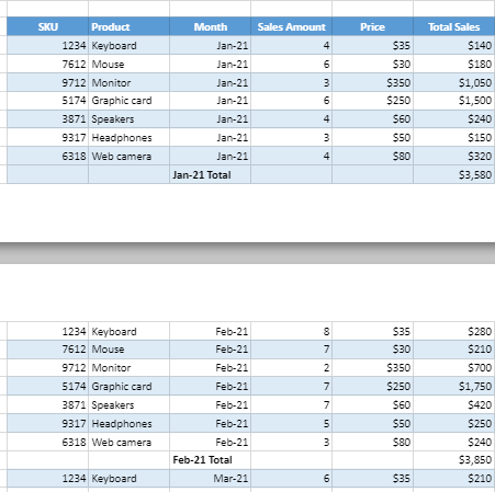
When you confirm and get back to the Print settings screen, you can see that every month is print on a separate page, so you set page breaks successfully.

Remove Page Breaks in Google Sheets

To remove page breaks, follow these steps on the Print settings page (CTRL + P):

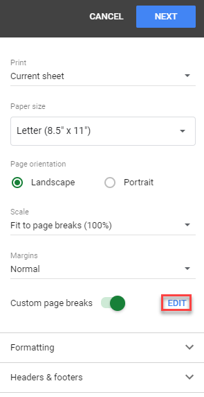
1. First click on the Edit button on the right side.

 

 

2. In the next window, position the cursor on the page break line you want to remove and click on the X sign which appears at the beginning of the line.

 

 

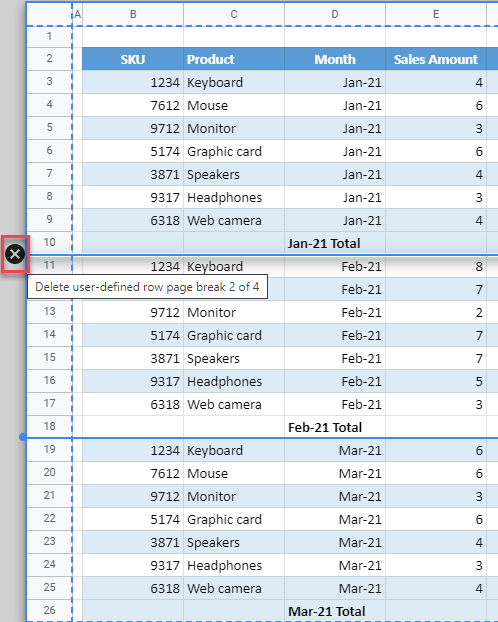
3. After that, the page break between Rows 10 and 11 is deleted. Click Confirm Breaks in the top right corner of the window.

 

 

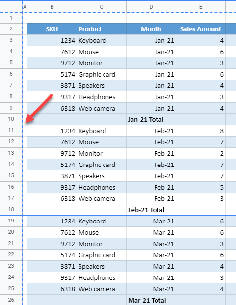
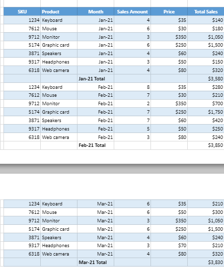
Finally, in the page settings, Jan-21 and Feb-21 rows are now on the first page while Mar-21 is on the second page since you didn’t move the second page break.

 

 

Remove All Page Breaks

To remove all custom page breaks, toggle the button next to Custom page breaks to turn it off.